Cluster variograms of multiple features

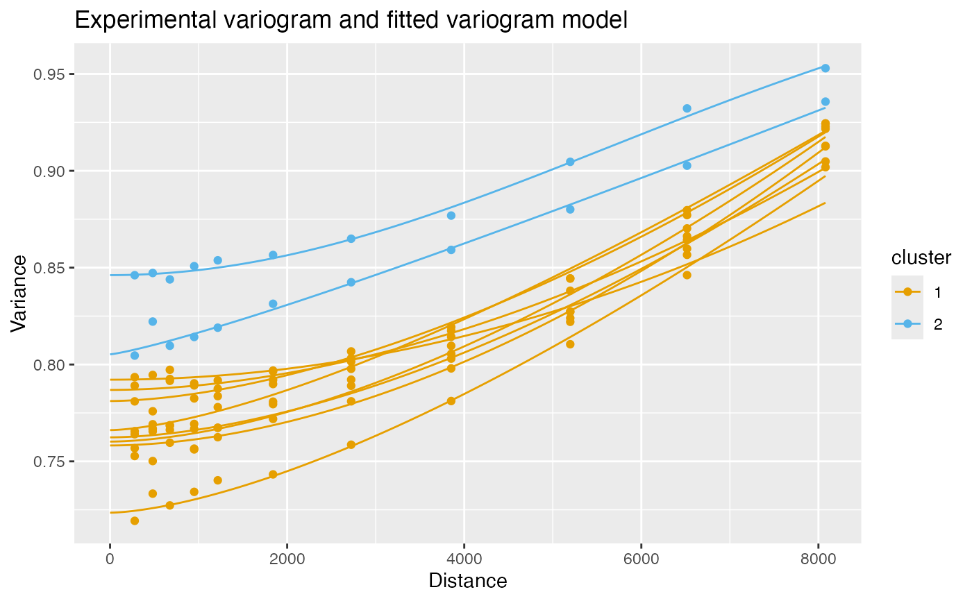
This function clusters variograms of features across samples to find patterns in decays in spatial autocorrelation. The fitted variograms are clustered as different samples can have different distance bins.

Usage

clusterVariograms(
  sfe,
  features,
  BLUSPARAM,
  n = 20,
  sample_id = "all",
  colGeometryName = NULL,
  annotGeometryName = NULL,
  reducedDimName = NULL,
  swap_rownames = NULL,
  name = "variogram"
)

Arguments

sfe

A SpatialFeatureExperiment object with correlograms computed for features of interest.

features

Features whose correlograms to cluster.

BLUSPARAM

A BlusterParam object specifying the algorithm to use.

n

Number of points on the fitted variogram line.

sample_id

Sample(s) in the SFE object whose cells/spots to use. Can be "all" to compute metric for all samples; the metric is computed separately for each sample.

colGeometryName

Name of colGeometry from which to look for features.

annotGeometryName

Name of annotGeometry from which to look for features.

reducedDimName

Name of a dimension reduction, can be seen in reducedDimNames. colGeometryName and annotGeometryName have precedence over reducedDimName.

swap_rownames

Column name of rowData(object) to be used to identify features instead of rownames(object) when labeling plot elements. If not found in rowData, then rownames of the gene count matrix will be used.

name

Name under which the correlogram results are stored, which is by default "sp.correlogram".

Value

A data frame with 3 columns: feature for the features,

cluster a factor for cluster membership of the features within each sample, and sample_id for the sample.

Examples

library(SFEData)
library(scater)
library(bluster)
library(Matrix)
#> 
#> Attaching package: ‘Matrix’
#> The following object is masked from ‘package:S4Vectors’:
#> 
#>     expand
sfe <- McKellarMuscleData()
#> see ?SFEData and browseVignettes('SFEData') for documentation
#> loading from cache
sfe <- logNormCounts(sfe)
# Just the highly expressed genes
gs <- order(Matrix::rowSums(counts(sfe)), decreasing = TRUE)[1:10]
genes <- rownames(sfe)[gs]

sfe <- runUnivariate(sfe, "variogram", features = genes)
clusts <- clusterVariograms(sfe, genes, BLUSPARAM = HclustParam(),
swap_rownames = "symbol")

# Plot the clustering
plotVariogram(sfe, genes, color_by = clusts, group = "feature",
use_lty = FALSE, swap_rownames = "symbol", show_np = FALSE)