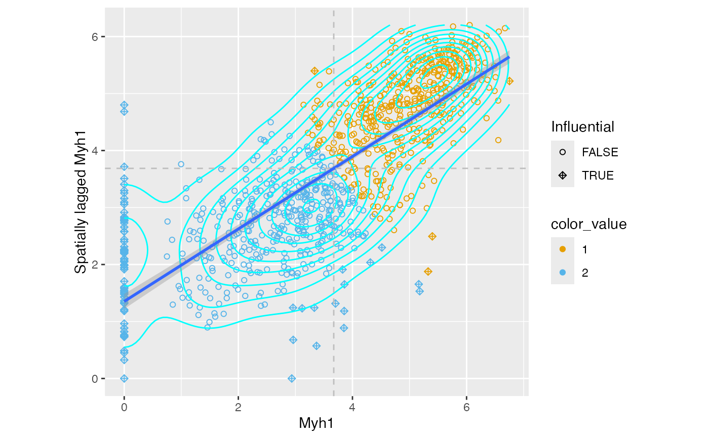
Use ggplot to plot the moran.plot results

This function uses ggplot2 to plot the Moran plot. The plot would be more aesthetically pleasing than the base R version implemented in spdep. In addition, contours are plotted to show point density on the plot, and the points can be colored by a variable, such as clusters. The contours may also be filled and only influential points plotted. When filled, the viridis E option is used.

Usage

moranPlot(
  sfe,
  feature,
  graphName = 1L,
  sample_id = "all",
  contour_color = "cyan",
  color_by = NULL,
  colGeometryName = NULL,
  annotGeometryName = NULL,
  plot_singletons = TRUE,
  binned = FALSE,
  filled = FALSE,
  divergent = FALSE,
  diverge_center = NULL,
  swap_rownames = NULL,
  bins = 100,
  binwidth = NULL,
  hex = FALSE,
  plot_influential = TRUE,
  bins_contour = NULL,
  name = "moran.plot",
  ...
)

Arguments

sfe: A SpatialFeatureExperiment object.
feature: Name of one variable to show on the plot. It will be converted to sentence case on the x axis and lower case in the y axis appended after "Spatially lagged". One feature at a time since the colors in color_by may be specific to this feature (e.g. from clusterMoranPlot).
graphName: Name of the colGraph or annotGraph, the spatial neighborhood graph used to compute the Moran plot. This is to determine which points are singletons to plot differently on this plot.
sample_id: One sample_id for the sample whose graph to plot.
contour_color: Color of the point density contours, which can be changed so the contours stand out from the points.
color_by: Variable to color the points by. It can be the name of a column in colData, a gene, or the name of a column in the colGeometry specified in colGeometryName. Or it can be a vector of the same length as the number of cells/spots in the sample_id of interest.
colGeometryName: Name of a colGeometry sf data frame whose numeric columns of interest are to be used to compute the metric. Use colGeometryNames to look up names of the sf data frames associated with cells/spots.
annotGeometryName: Name of a annotGeometry of the SFE object, to annotate the gene expression plot.
plot_singletons: Logical, whether to plot items that don't have spatial neighbors.
binned: Logical, whether to plot 2D histograms. This argument has precedence to filled.
filled: Logical, whether to plot filled contours for the non-influential points and only plot influential points as points.
divergent: Logical, whether a divergent palette should be used.
diverge_center: If divergent = TRUE, the center from which the palette should diverge. If NULL, then not centering.
swap_rownames: Column name of rowData(object) to be used to identify features instead of rownames(object) when labeling plot elements. If not found in rowData, then rownames of the gene count matrix will be used.
bins: If binning the colGeometry in space due to large number of cells or spots, the number of bins, passed to geom_bin2d or geom_hex. If NULL (default), then the colGeometry is plotted without binning. If binning, a point geometry is recommended. If the geometry is not point, then the centroids will be used.
binwidth: Width of bins, passed to geom_bin2d or geom_hex.
hex: Logical, whether to use geom_hex. Note that geom_hex is broken in ggplot2 version 3.4.0. Please update ggplot2 if you are getting horizontal stripes when hex = TRUE.
plot_influential: Logical, whether to plot influential points with different palette if binned = TRUE.
bins_contour: Number of bins in the point density contour. Use a smaller number to make sparser contours.
name: Name under which the Moran plot results are stored. By default "moran.plot".
...: Other arguments to pass to geom_density2d.

Value

A ggplot object.

Examples

library(SpatialFeatureExperiment)
library(SingleCellExperiment)
library(SFEData)
library(bluster)
library(scater)
sfe <- McKellarMuscleData("full")
#> see ?SFEData and browseVignettes('SFEData') for documentation
#> loading from cache
sfe <- sfe[, colData(sfe)$in_tissue]
sfe <- logNormCounts(sfe)
colGraph(sfe, "visium") <- findVisiumGraph(sfe)
sfe <- runUnivariate(sfe, type = "moran.plot", features = "Myh1",
                     swap_rownames = "symbol")
clust <- clusterMoranPlot(sfe, "Myh1", BLUSPARAM = KmeansParam(2),
                          swap_rownames = "symbol")
moranPlot(sfe, "Myh1", graphName = "visium", color_by = clust[, 1],
          swap_rownames = "symbol")