Plot correlogram

Use ggplot2 to plot correlograms computed by runUnivariate, pulling results from rowData. Correlograms of multiple genes with error bars can be plotted, and they can be colored by any numeric or categorical column in rowData or a vector with the same length as nrow of the SFE object. The coloring is useful when the correlograms are clustered to show types of length scales or patterns of decay of spatial autocorrelation. For method = "I", the error bars are twice the standard deviation of the estimated Moran's I value.

Usage

plotCorrelogram(
  sfe,
  features,
  sample_id = "all",
  method = "I",
  color_by = NULL,
  facet_by = c("sample_id", "features"),
  ncol = NULL,
  colGeometryName = NULL,
  annotGeometryName = NULL,
  reducedDimName = NULL,
  plot_signif = TRUE,
  p_adj_method = "BH",
  divergent = FALSE,
  diverge_center = NULL,
  swap_rownames = NULL,
  name = "sp.correlogram"
)

Arguments

sfe

A SpatialFeatureExperiment object.

features

Features to plot, must be in rownames of the gene count matrix, colnames of colData or a colGeometry, colnames of cell embeddings in reducedDim, or numeric indices of dimension reduction components.

sample_id

Sample(s) in the SFE object whose cells/spots to use. Can be "all" to compute metric for all samples; the metric is computed separately for each sample.

method

"corr" for correlation, "I" for Moran's I, "C" for Geary's C

color_by

Name of a column in rowData(sfe) or in the featureData of colData (see colFeatureData), colGeometry, or annotGeometry by which to color the correlogram of each feature. Alternatively, a vector of the same length as features, or a data frame from clusterCorrelograms.

facet_by

Whether to facet by sample_id (default) or features. If facetting by sample_id, then different features will be plotted in the same facet for comparison. If facetting by features, then different samples will be compared for each feature. Ignored if only one sample is specified.

ncol

Number of columns if facetting.

colGeometryName

Name of a colGeometry sf data frame whose numeric columns of interest are to be used to compute the metric. Use colGeometryNames to look up names of the sf data frames associated with cells/spots.

annotGeometryName

Name of a annotGeometry of the SFE object, to annotate the gene expression plot.

reducedDimName

Name of a dimension reduction, can be seen in reducedDimNames. colGeometryName and annotGeometryName have precedence over reducedDimName.

plot_signif

Logical, whether to plot significance symbols: p < 0.001: ***, p < 0.01: **, p < 0.05 *, p < 0.1: ., otherwise no symbol. The p-values are two sided, based on the assumption that the estimated Moran's I is normally distributed with mean from a randomized version of the data. The mean and variance come from moran.test for Moran's I and geary.test for Geary's C. Take the results with a grain of salt if the data is not normally distributed.

p_adj_method

Multiple testing correction method as in p.adjust, to correct for multiple testing (number of lags times number of features) in the Moran's I estimates if plot_signif = TRUE.

divergent

Logical, whether a divergent palette should be used.

diverge_center

If divergent = TRUE, the center from which the palette should diverge. If NULL, then not centering.

swap_rownames

Column name of rowData(object) to be used to identify features instead of rownames(object) when labeling plot elements. If not found in rowData, then rownames of the gene count matrix will be used.

name

Name under which the correlogram results are stored, which is by default "sp.correlogram".

Value

A ggplot object.

Examples

library(SpatialFeatureExperiment)
library(SFEData)
library(bluster)
library(scater)
sfe <- McKellarMuscleData("small")
#> see ?SFEData and browseVignettes('SFEData') for documentation
#> loading from cache
sfe <- logNormCounts(sfe)
colGraph(sfe, "visium") <- findVisiumGraph(sfe)
inds <- c(1, 3, 4, 5)
features <- rownames(sfe)[inds]
sfe <- runUnivariate(sfe,
    type = "sp.correlogram", features = features,
    exprs_values = "counts", order = 5
)
clust <- clusterCorrelograms(sfe,
    features = features,
    BLUSPARAM = KmeansParam(2)
)
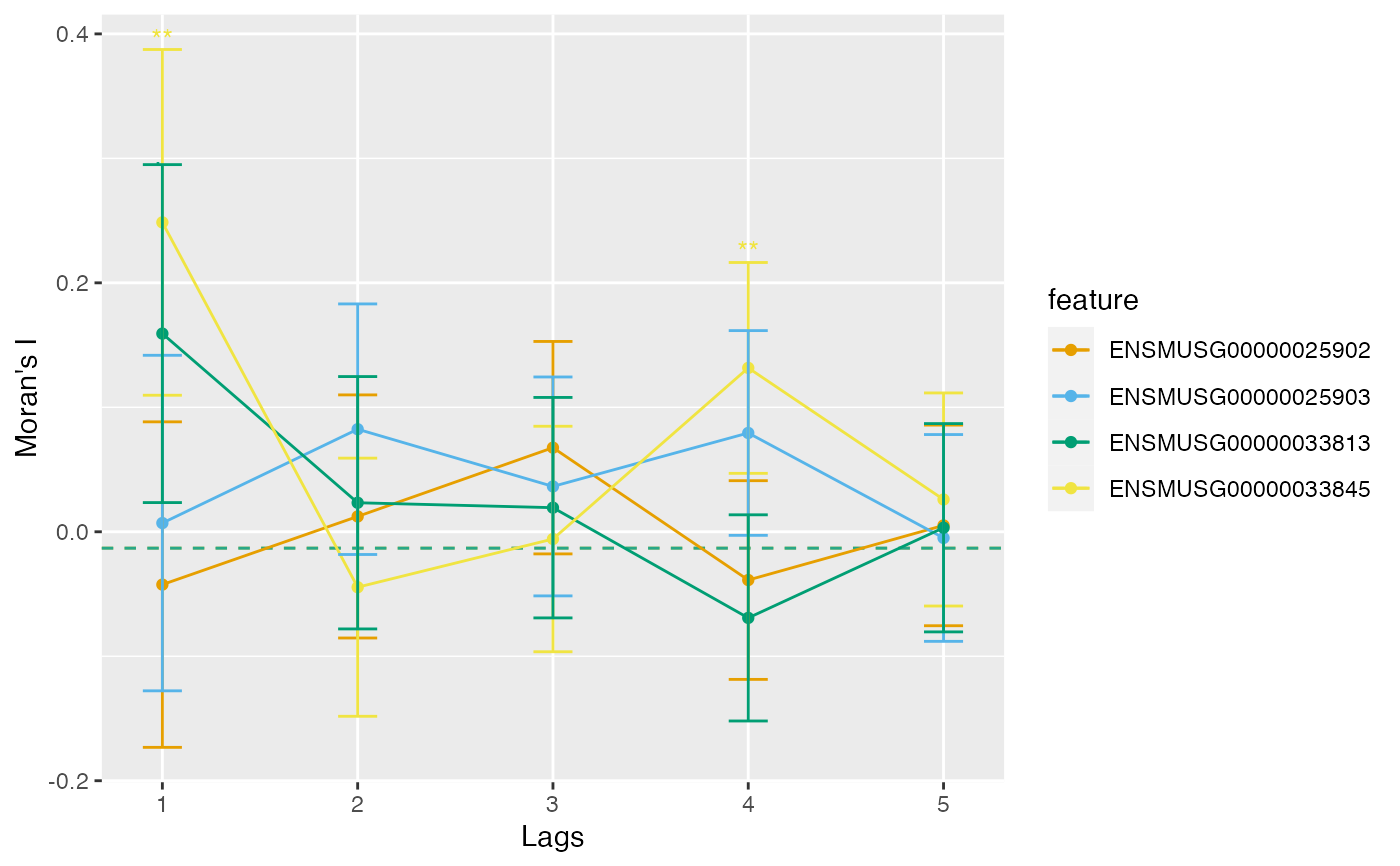
# Color by features
plotCorrelogram(sfe, features)

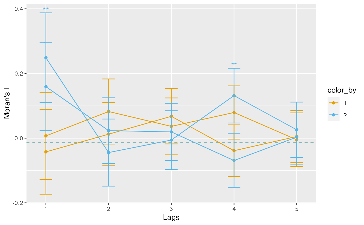
# Color by something else
plotCorrelogram(sfe, features, color_by = clust$cluster)

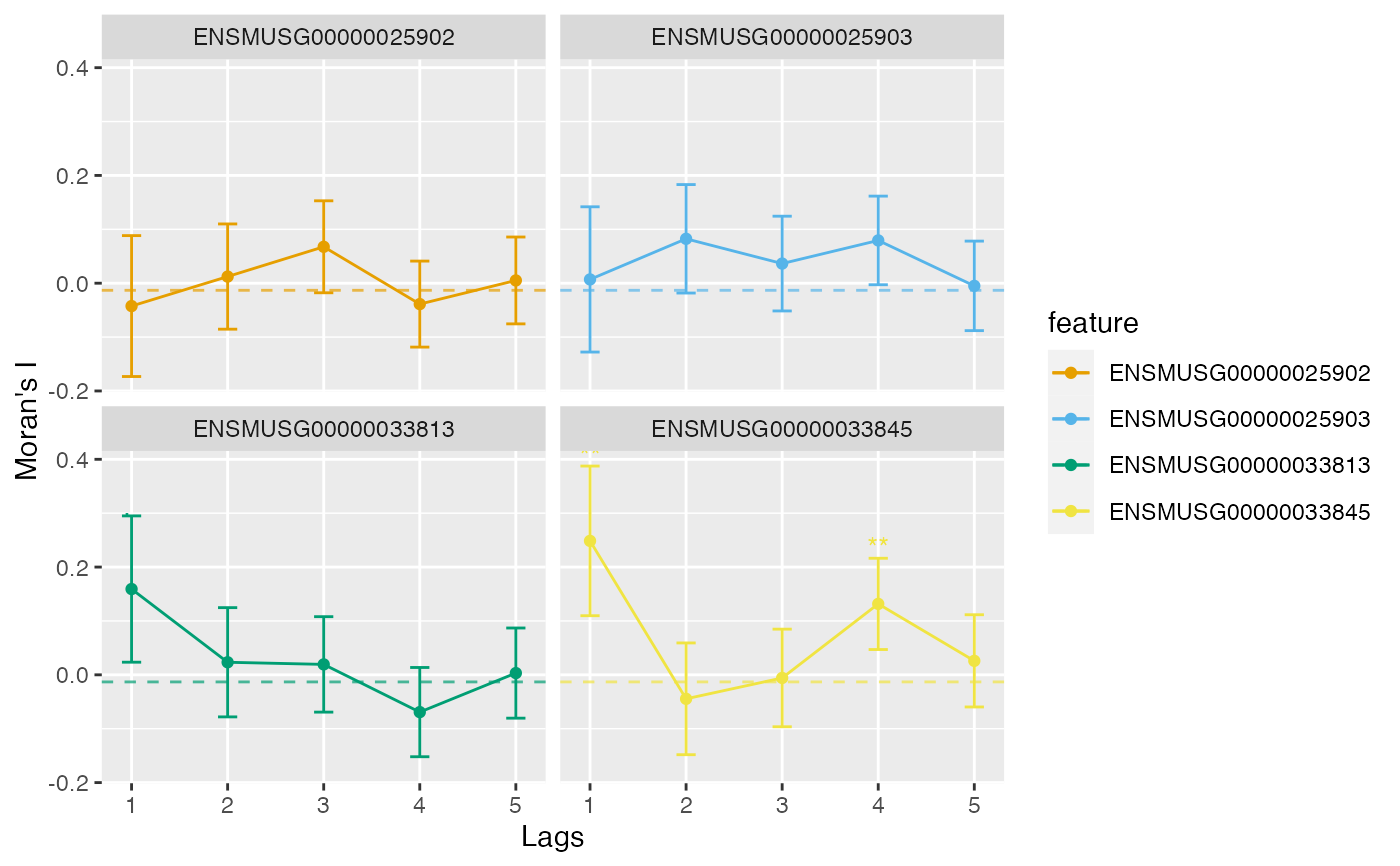
# Facet by features
plotCorrelogram(sfe, features, facet_by = "features")