Plot gene expression in space — plotSpatialFeature • Voyager

Unlike Seurat and ggspavis, plotting functions in this package uses geom_sf whenever applicable.

Usage

plotSpatialFeature(
  sfe,
  features,
  colGeometryName = 1L,
  sample_id = "all",
  ncol = NULL,
  ncol_sample = NULL,
  annotGeometryName = NULL,
  rowGeometryName = NULL,
  rowGeometryFeatures = NULL,
  annot_aes = list(),
  annot_fixed = list(),
  tx_fixed = list(),
  exprs_values = "logcounts",
  bbox = NULL,
  tx_file = NULL,
  image_id = NULL,
  channel = NULL,
  maxcell = 5e+05,
  aes_use = c("fill", "color", "shape", "linetype"),
  divergent = FALSE,
  diverge_center = NA,
  annot_divergent = FALSE,
  annot_diverge_center = NA,
  size = 0.5,
  shape = 16,
  linewidth = 0,
  linetype = 1,
  alpha = 1,
  color = "black",
  fill = "gray80",
  swap_rownames = NULL,
  scattermore = FALSE,
  pointsize = 0,
  bins = NULL,
  summary_fun = sum,
  hex = FALSE,
  show_axes = FALSE,
  dark = FALSE,
  palette = colorRampPalette(c("black", "white"))(255),
  normalize_channels = FALSE,
  ...
)

Arguments

sfe: A SpatialFeatureExperiment object.
features: Features to plot, must be in rownames of the gene count matrix, colnames of colData or a colGeometry.
colGeometryName: Name of a colGeometry sf data frame whose numeric columns of interest are to be used to compute the metric. Use colGeometryNames to look up names of the sf data frames associated with cells/spots.
sample_id: Sample(s) in the SFE object whose cells/spots to use. Can be "all" to compute metric for all samples; the metric is computed separately for each sample.
ncol: Number of columns if plotting multiple features. Defaults to NULL, which means using the same logic as facet_wrap, which is used by patchwork's wrap_plots by default.
ncol_sample: If plotting multiple samples as facets, how many columns of such facets. This is distinct from ncols, which is for multiple features. When plotting multiple features for multiple samples, then the result is a multi-panel plot each panel of which is a plot for each feature facetted by samples.
annotGeometryName: Name of a annotGeometry of the SFE object, to annotate the gene expression plot.
rowGeometryName: Name of a rowGeometry of the SFE object to plot.
rowGeometryFeatures: Which features from rowGeometry to plot. Can only be a small number to avoid overplotting. Different features are distinguished by point shape. By default (NULL), when rowGeometryName is specified, this will be whichever items in features that are also in the row names of the SFE object. If features specified for this argument are not the same as or a subset of those in argument features, then the spots of all features specified here will be plotted, differentiated by point shape.
annot_aes: A named list of plotting parameters for the annotation sf data frame. The names are which geom (as in ggplot2, such as color and fill), and the values are column names in the annotation sf data frame. Tidyeval is NOT supported.
annot_fixed: Similar to annot_aes, but for fixed aesthetic settings, such as color = "gray". The defaults are the same as the relevant defaults for this function.
tx_fixed: Similar to annot_fixed, but to specify fixed aesthetic for transcript spots.
exprs_values: Integer scalar or string indicating which assay of x contains the expression values.
bbox: A bounding box to specify a smaller region to plot, useful when the dataset is large. Can be a named numeric vector with names "xmin", "xmax", "ymin", and "ymax", in any order. If plotting multiple samples, it should be a matrix with sample IDs as column names and "xmin", "ymin", "xmax", and "ymax" as row names. If multiple samples are plotted but bbox is a vector rather than a matrix, then the same bounding box will be used for all samples. You may see points at the edge of the geometries if the intersection between the bounding box and a geometry happens to be a point there. If NULL, then the entire tissue is plotted.
tx_file: File path to GeoParquet file of the transcript spots if you don't wish to load all transcript spots into the SFE object. See formatTxSpots on generating such a GeoParquet file.
image_id: ID of the image to plot behind the geometries. If NULL, then not plotting images. Use imgData to see image IDs present. To plot multiple grayscale images as different RGB channels, use a named vector here, whose names are channel names (r, g, b), and values are image_ids of the corresponding images. The RGB colorization may not be colorblind friendly. When plotting multiple samples, it is assumed that the same image_id is used for each channel across different samples.
channel: Numeric vector indicating which channels in a multi-channel image to plot. If NULL, grayscale is plotted if there is 1 channel and RGB for the first 3 channels. The numeric vector can be named (r, g, b) to indicate which channel maps to which color. The RGB colorization may not be colorblind friendly. This argument cannot be specified while image_id is a named vector to plot different grayscale images as different channels.
maxcell: Maximum number of pixels to plot in the image. If the image is larger, it will be resampled so it have less than this number of pixels to save memory and for faster plotting. We recommend reducing this number when plotting multiple facets.
aes_use: Aesthetic to use for discrete variables. For continuous variables, it's always "fill" for polygons and point shapes 21-25. For discrete variables, it can be fill, color, shape, or linetype, whenever applicable. The specified value will be changed to the applicable equivalent. For example, if the geometry is point but "linetype" is specified, then "shaped" will be used instead.
divergent: Logical, whether a divergent palette should be used.
diverge_center: If divergent = TRUE, the center from which the palette should diverge. If NULL, then not centering.
annot_divergent: Just as divergent, but for the annotGeometry in case it's different.
annot_diverge_center: Just as diverge_center, but for the annotGeometry in case it's different.
size: Fixed size of points. For points defaults to 0.5. Ignored if size_by is specified.
shape: Fixed shape of points, ignored if shape_by is specified and applicable.
linewidth: Width of lines, including outlines of polygons. For polygons, this defaults to 0, meaning no outlines.
linetype: Fixed line type, ignored if linetype_by is specified and applicable.
alpha: Transparency.
color: Fixed color for colGeometry if color_by is not specified or not applicable, or for annotGeometry if annot_color_by is not specified or not applicable.
fill: Similar to color, but for fill.
swap_rownames: Column name of rowData(object) to be used to identify features instead of rownames(object) when labeling plot elements. If not found in rowData, then rownames of the gene count matrix will be used.
scattermore: Logical, whether to use the scattermore package to greatly speed up plotting numerous points. Only used for POINT colGeometries. If the geometry is not POINT, then the centroids are used. Recommended for plotting hundreds of thousands or more cells where the cell polygons can't be seen when plotted due to the large number of cells and small plot size such as when plotting multiple panels for multiple features.
pointsize: Radius of rasterized point in scattermore. Default to 0 for single pixels (fastest).
bins: If binning the colGeometry in space due to large number of cells or spots, the number of bins, passed to geom_bin2d or geom_hex. If NULL (default), then the colGeometry is plotted without binning. If binning, a point geometry is recommended. If the geometry is not point, then the centroids will be used.
summary_fun: Function to summarize the feature value when the colGeometry is binned.
hex: Logical, whether to use geom_hex. Note that geom_hex is broken in ggplot2 version 3.4.0. Please update ggplot2 if you are getting horizontal stripes when hex = TRUE.
show_axes: Logical, whether to show axes.
dark: Logical, whether to use dark theme. When using dark theme, the palette will have lighter color represent higher values as if glowing in the dark. This is intended for plotting gene expression on top of fluorescent images.
palette: Vector of colors to use to color grayscale images.
normalize_channels: Logical, whether to normalize each channel of the image individually. Should be FALSE for bright field color images such as H&E but should set to TRUE for fluorescent images.
...: Other arguments passed to wrap_plots.

Value

A ggplot2 object if plotting one feature. A patchwork object if plotting multiple features.

Details

In the documentation of this function, a "feature" can be a gene (or whatever entity that corresponds to rows of the gene count matrix), a column in colData, or a column in the colGeometry sf data frame specified in the colGeometryName argument.

In the light theme, for continuous variables, the Blues palette from colorbrewer is used if divergent = FALSE, and the roma palette from the scico package if divergent = TRUE. In the dark theme, the nuuk palette from scico is used if divergent = FALSE, and the berlin palette from scico is used if divergent = TRUE. For discrete variables, the dittoSeq palette is used.

For annotation, the YlOrRd colorbrewer palette is used for continuous variables in the light theme. In the dark theme, the acton palette from scico is used when divergent = FALSE and the vanimo palette from scico is used when divergent = FALSE. The other end of the dittoSeq palette is used for discrete variables.

Each individual palette should be colorblind friendly, but when plotting continuous variables coloring a colGeometry and a annotGeometry simultaneously, the combination of the two palettes is not guaranteed to be colorblind friendly.

In addition, when plotting an image behind the geometries, the colors of the image may distort color perception of the values of the geometries.

theme_void is used for all spatial plots in this package, because the units in the spatial coordinates are often arbitrary. This can be overriden to show the axes by using a different theme as normally done in ggplot2.

Examples

library(SFEData)
library(sf)
sfe <- McKellarMuscleData("small")
#> see ?SFEData and browseVignettes('SFEData') for documentation
#> loading from cache
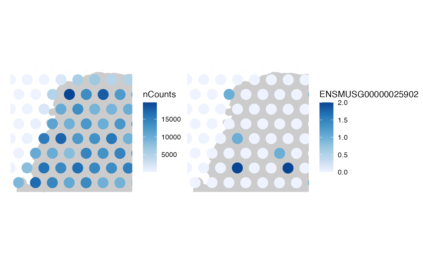
# features can be genes or colData or colGeometry columns
plotSpatialFeature(sfe, c("nCounts", rownames(sfe)[1]),
    exprs_values = "counts",
    colGeometryName = "spotPoly",
    annotGeometryName = "tissueBoundary"
)

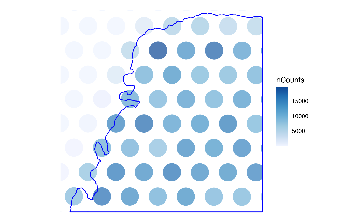
# Change fixed aesthetics
plotSpatialFeature(sfe, "nCounts",
    colGeometryName = "spotPoly",
    annotGeometryName = "tissueBoundary",
    annot_fixed = list(color = "blue", size = 0.3, fill = NA),
    alpha = 0.7
)

# Make the myofiber segmentations a valid POLYGON geometry
ag <- annotGeometry(sfe, "myofiber_simplified")
ag <- st_buffer(ag, 0)
ag <- ag[!st_is_empty(ag), ]
annotGeometry(sfe, "myofiber_simplified") <- ag
# Also plot an annotGeometry variable
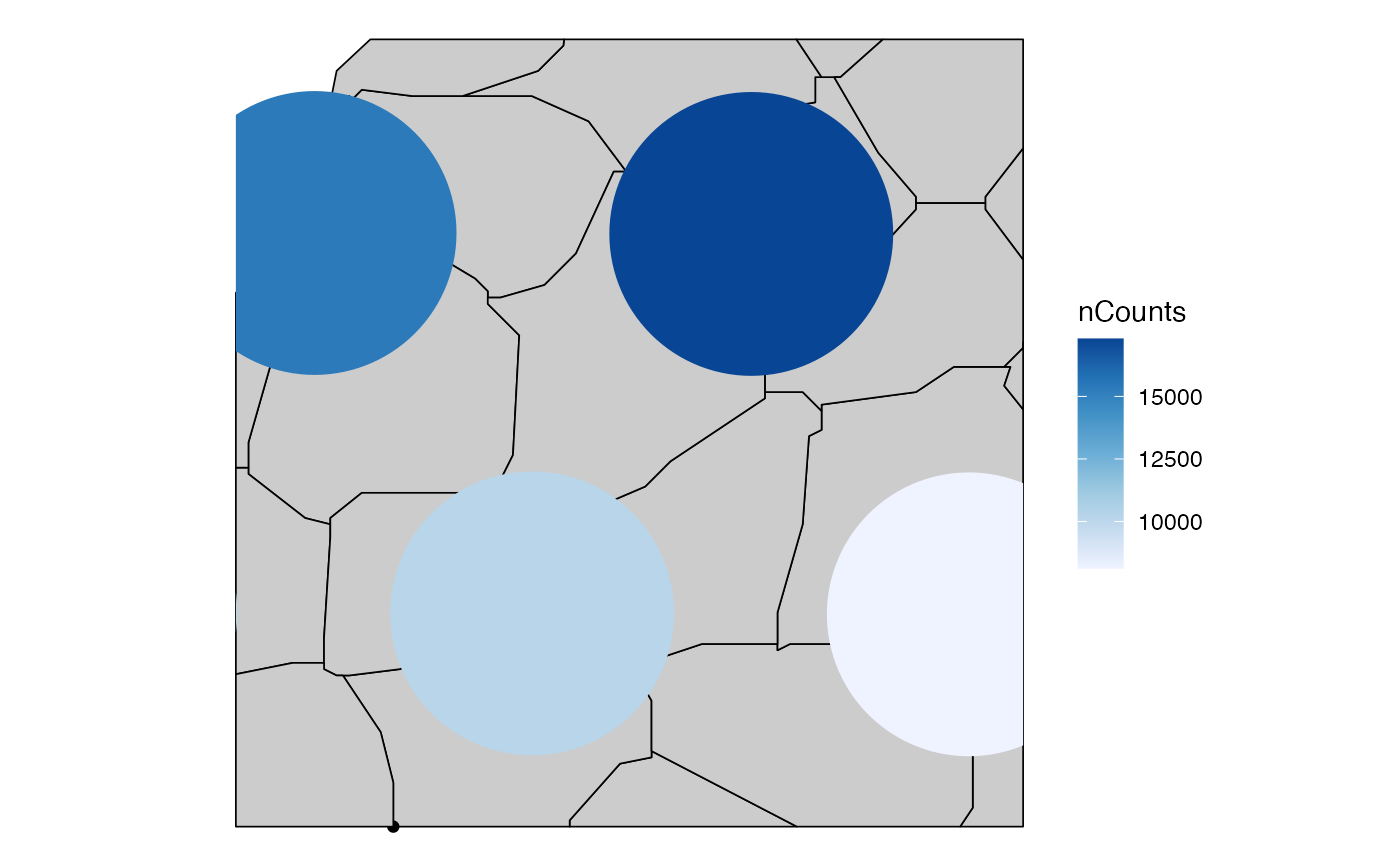
plotSpatialFeature(sfe, "nCounts",
    colGeometryName = "spotPoly",
    annotGeometryName = "myofiber_simplified",
    annot_aes = list(fill = "area")
)

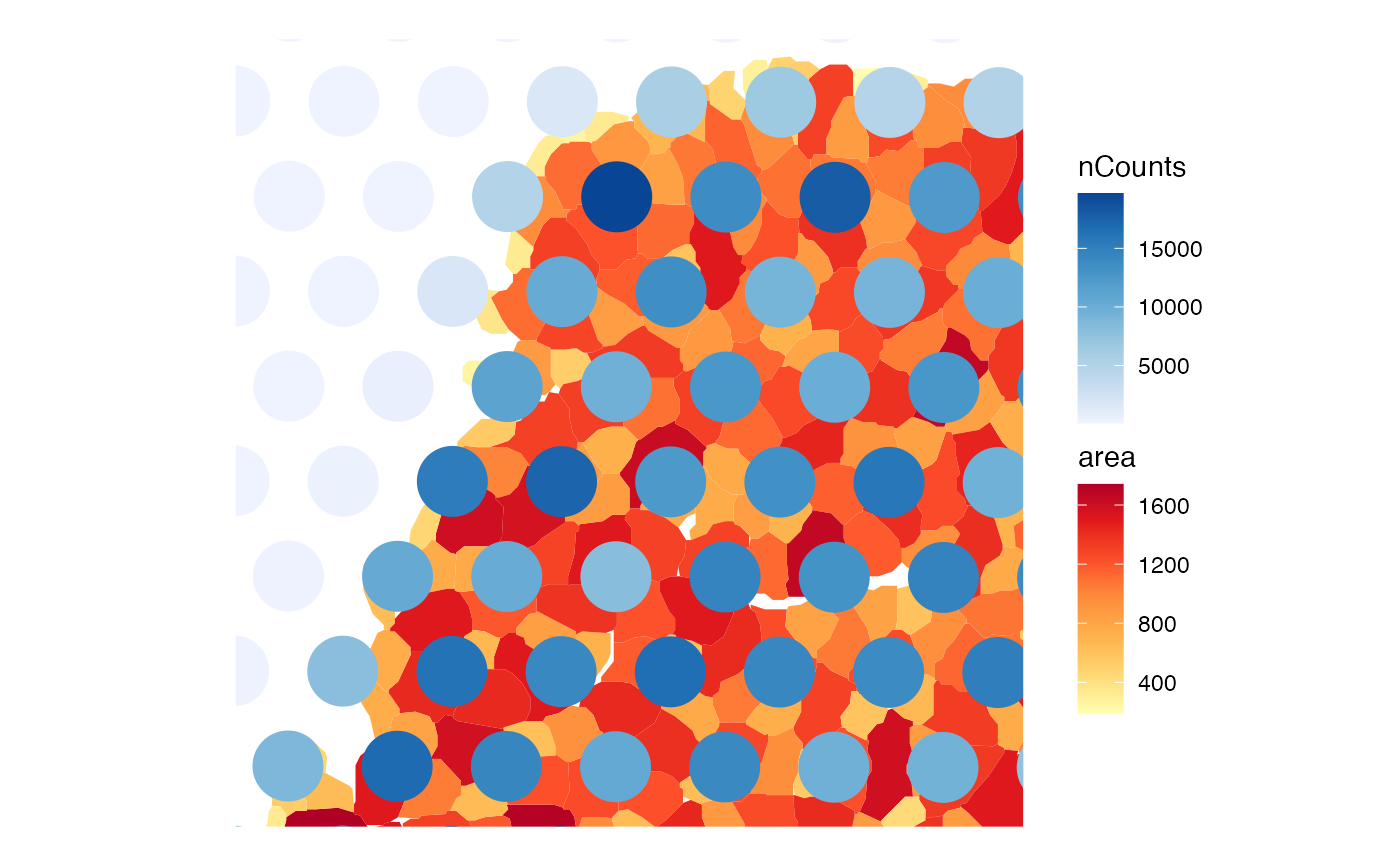# Use a bounding box to zoom in
bbox <- c(xmin = 5500, ymin = 13500, xmax = 6000, ymax = 14000)
plotSpatialFeature(sfe, "nCounts", colGeometryName = "spotPoly",
                  annotGeometry = "myofiber_simplified",
                  bbox = bbox, annot_fixed = list(linewidth = 0.3))