Plot local results — plotLocalResult • Voyager

Plot results of local spatial analyses in space, such as local Getis-Ord Gi* values.

Usage

plotLocalResult(
  sfe,
  name,
  features,
  attribute = NULL,
  sample_id = "all",
  colGeometryName = NULL,
  annotGeometryName = NULL,
  ncol = NULL,
  ncol_sample = NULL,
  annot_aes = list(),
  annot_fixed = list(),
  bbox = NULL,
  image_id = NULL,
  maxcell = 5e+05,
  aes_use = c("fill", "color", "shape", "linetype"),
  divergent = FALSE,
  diverge_center = NULL,
  annot_divergent = FALSE,
  annot_diverge_center = NULL,
  size = 0.5,
  shape = 16,
  linewidth = 0,
  linetype = 1,
  alpha = 1,
  color = "black",
  fill = "gray80",
  swap_rownames = NULL,
  scattermore = FALSE,
  pointsize = 0,
  bins = NULL,
  summary_fun = sum,
  hex = FALSE,
  dark = FALSE,
  type = name,
  ...
)

Arguments

sfe: A SpatialFeatureExperiment object.
name: Which local spatial results. Use localResultNames to see which types of results have already been calculated.
features: Character vector of vectors. To see which features have the results of a given type, see localResultFeatures.
attribute: Which field in the local results of the type and features. If the result of each feature is a vector, the this argument is ignored. But if the result is a data frame or a matrix, then this is the column name of the result, such as "Ii" for local Moran's I. For each local spatial analysis method, there's a default attribute. See Details. Use localResultAttrs.
sample_id: Sample(s) in the SFE object whose cells/spots to use. Can be "all" to compute metric for all samples; the metric is computed separately for each sample.
colGeometryName: Name of a colGeometry sf data frame whose numeric columns of interest are to be used to compute the metric. Use colGeometryNames to look up names of the sf data frames associated with cells/spots.
annotGeometryName: Name of a annotGeometry of the SFE object, to annotate the gene expression plot.
ncol: Number of columns if plotting multiple features. Defaults to NULL, which means using the same logic as facet_wrap, which is used by patchwork's wrap_plots by default.
ncol_sample: If plotting multiple samples as facets, how many columns of such facets. This is distinct from ncols, which is for multiple features. When plotting multiple features for multiple samples, then the result is a multi-panel plot each panel of which is a plot for each feature facetted by samples.
annot_aes: A named list of plotting parameters for the annotation sf data frame. The names are which geom (as in ggplot2, such as color and fill), and the values are column names in the annotation sf data frame. Tidyeval is NOT supported.
annot_fixed: Similar to annot_aes, but for fixed aesthetic settings, such as color = "gray". The defaults are the same as the relevant defaults for this function.
bbox: A bounding box to specify a smaller region to plot, useful when the dataset is large. Can be a named numeric vector with names "xmin", "xmax", "ymin", and "ymax", in any order. If plotting multiple samples, it should be a matrix with sample IDs as column names and "xmin", "ymin", "xmax", and "ymax" as row names. If multiple samples are plotted but bbox is a vector rather than a matrix, then the same bounding box will be used for all samples. You may see points at the edge of the geometries if the intersection between the bounding box and a geometry happens to be a point there. If NULL, then the entire tissue is plotted.
image_id: ID of the image to plot behind the geometries. If NULL, then not plotting images. Use imgData to see image IDs present.
maxcell: Maximum number of pixels to plot in the image. If the image is larger, it will be resampled so it have less than this number of pixels to save memory and for faster plotting. We recommend reducing this number when plotting multiple facets.
aes_use: Aesthetic to use for discrete variables. For continuous variables, it's always "fill" for polygons and point shapes 21-25. For discrete variables, it can be fill, color, shape, or linetype, whenever applicable. The specified value will be changed to the applicable equivalent. For example, if the geometry is point but "linetype" is specified, then "shaped" will be used instead.
divergent: Logical, whether a divergent palette should be used.
diverge_center: If divergent = TRUE, the center from which the palette should diverge. If NULL, then not centering.
annot_divergent: Just as divergent, but for the annotGeometry in case it's different.
annot_diverge_center: Just as diverge_center, but for the annotGeometry in case it's different.
size: Fixed size of points. For points defaults to 0.5. Ignored if size_by is specified.
shape: Fixed shape of points, ignored if shape_by is specified and applicable.
linewidth: Width of lines, including outlines of polygons. For polygons, this defaults to 0, meaning no outlines.
linetype: Fixed line type, ignored if linetype_by is specified and applicable.
alpha: Transparency.
color: Fixed color for colGeometry if color_by is not specified or not applicable, or for annotGeometry if annot_color_by is not specified or not applicable.
fill: Similar to color, but for fill.
swap_rownames: Column name of rowData(object) to be used to identify features instead of rownames(object) when labeling plot elements. If not found in rowData, then rownames of the gene count matrix will be used.
scattermore: Logical, whether to use the scattermore package to greatly speed up plotting numerous points. Only used for POINT colGeometries. If the geometry is not POINT, then the centroids are used. Recommended for plotting hundreds of thousands or more cells where the cell polygons can't be seen when plotted due to the large number of cells and small plot size such as when plotting multiple panels for multiple features.
pointsize: Radius of rasterized point in scattermore. Default to 0 for single pixels (fastest).
bins: If binning the colGeometry in space due to large number of cells or spots, the number of bins, passed to geom_bin2d or geom_hex. If NULL (default), then the colGeometry is plotted without binning. If binning, a point geometry is recommended. If the geometry is not point, then the centroids will be used.
summary_fun: Function to summarize the feature value when the colGeometry is binned.
hex: Logical, whether to use geom_hex. Note that geom_hex is broken in ggplot2 version 3.4.0. Please update ggplot2 if you are getting horizontal stripes when hex = TRUE.
dark: Logical, whether to use dark theme. When using dark theme, the palette will have lighter color represent higher values as if glowing in the dark. This is intended for plotting gene expression on top of fluorescent images.
type: An SFEMethod object or a string corresponding to the name of one of such objects in the environment. If the localResult of interest was manually added outside runUnivariate and runBivariate, so the method is not recorded, then the type argument can be used to specify the method to properly get the title and labels. By default, this argument is set to be the same as argument name. If the method parameters are recorded, then the type argument is ignored.
...: Other arguments passed to wrap_plots.

Value

A ggplot2 object if plotting one feature. A patchwork

object if plotting multiple features.

Details

Many local spatial analyses return a data frame or matrix as the results, whose columns can be the statistic of interest at each location, its variance, expected value from permutation, p-value, and etc. The attribute argument specifies which column to use when there are multiple columns. Below are the defaults for each local method supported by this package what what they mean:

localmoran and localmoran_perm: Ii, local Moran's I statistic at each location.
localC_perm: localC, the local Geary C statistic at each location.
localG and localG_perm: localG, the local Getis-Ord Gi or Gi* statistic. If include_self = TRUE when calculateUnivariate or runUnivariate was called, then it would be Gi*. Otherwise it's Gi.
LOSH and LOSH.mc: Hi, local spatial heteroscedasticity
moran.plot: wx, the average of the value of each neighbor of each location. Moran plot is best plotted as a scatter plot of wx vs x. See moranPlot.

Other local methods not listed above return vectors as results. For instance, localC returns a vector by default, which is the local Geary's C statistic.

Note

While this function shares internals with plotSpatialFeature, there are some important differences. In plotSpatialFeature, the annotGeometry is indeed only used for annotation and the protagonist is the colGeometry, since it's easy to directly use ggplot2 to plot the data in annotGeometry sf data frames while overlaying annotGeometry and colGeometry involves more complicated code. In contrast, in this function, local results for annotGeometry can be plotted separately without anything related to colGeometry. Note that when annotGeometry local results are plotted without colGeometry, the annot_* arguments are ignored. Use the other arguments for aesthetics as if it's for colGeometry.

Examples

library(SpatialFeatureExperiment)
library(SFEData)
library(scater)
sfe <- McKellarMuscleData("small")
#> see ?SFEData and browseVignettes('SFEData') for documentation
#> loading from cache
sfe <- sfe[,sfe$in_tissue]
colGraph(sfe, "visium") <- findVisiumGraph(sfe)
feature_use <- rownames(sfe)[1]
sfe <- logNormCounts(sfe)
sfe <- runUnivariate(sfe, "localmoran", feature_use)
# Which types of results are available?
localResultNames(sfe)
#> [1] "localmoran"
# Which features for localmoran?
localResultFeatures(sfe, "localmoran")
#> [1] "ENSMUSG00000025902"
# Which columns does the localmoran results have?
localResultAttrs(sfe, "localmoran", feature_use)
#>  [1] "Ii"             "E.Ii"           "Var.Ii"         "Z.Ii"          
#>  [5] "Pr(z != E(Ii))" "mean"           "median"         "pysal"         
#>  [9] "-log10p"        "-log10p_adj"   
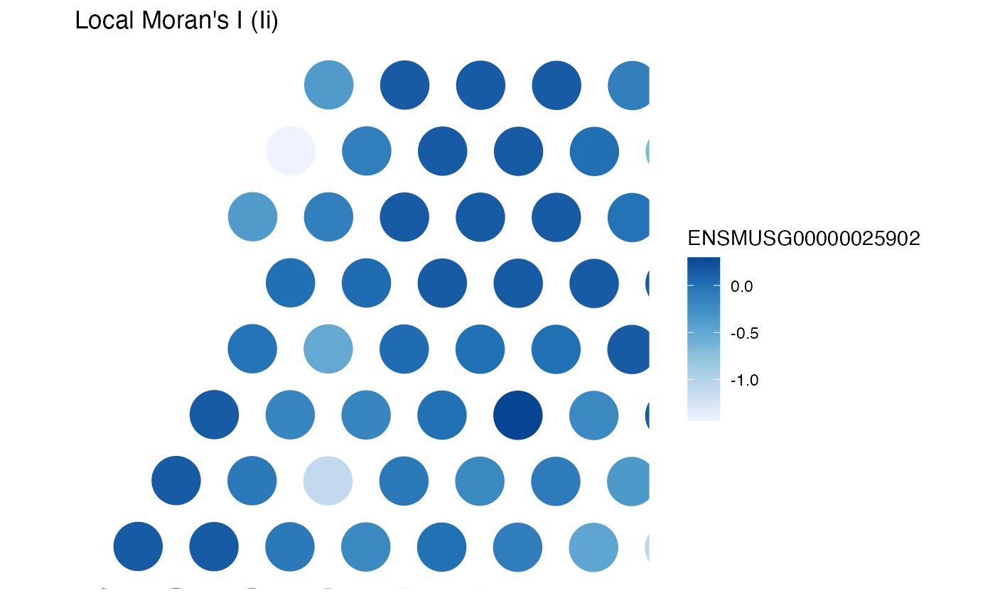
plotLocalResult(sfe, "localmoran", feature_use, "Ii",
    colGeometryName = "spotPoly"
)


# For annotGeometry
# Make sure it's type POLYGON
annotGeometry(sfe, "myofiber_simplified") <-
    sf::st_buffer(annotGeometry(sfe, "myofiber_simplified"), 0)
annotGraph(sfe, "poly2nb_myo") <-
    findSpatialNeighbors(sfe,
        type = "myofiber_simplified", MARGIN = 3,
        method = "poly2nb", zero.policy = TRUE
    )
sfe <- annotGeometryUnivariate(sfe, "localmoran",
    features = "area",
    annotGraphName = "poly2nb_myo",
    annotGeometryName = "myofiber_simplified",
    zero.policy = TRUE
)
plotLocalResult(sfe, "localmoran", "area", "Ii",
    annotGeometryName = "myofiber_simplified",
    size = 0.3, color = "cyan"
)

plotLocalResult(sfe, "localmoran", "area", "Z.Ii",
    annotGeometryName = "myofiber_simplified"
)

# don't use annot_* arguments when annotGeometry is plotted without colGeometry