5 Current era technologies

5.1 ROI selection

A simple way to preserve spatial information is to isolate the samples from known locations in the tissue, and the act of selection and isolation is the only means to preserve the locations. The samples can be isolated physically or by molecular techniques. The known locations can be targeted, for cells with certain histological characteristics, or untargeted, on a grid over the tissue.

5.1.1 History of LCM

5.1.1.1 Microdissection

LCM, also known as laser microdissection (LMD), is by far the most commonly used method of microdissection. Before LCM, manual microdissection could isolate small pieces of tissue, but the process was laborious (Bidarimath, Edwards, and Tayade 2015). Laser microdissection predates ISH, though it was not used for spatial transcriptomics until it was possible to profile the transcriptome from small quantity of tissue.

A precursor to laser microdissection is the 1912 “Strahlenstich”, which focused a conventional light source to a spot a few micrometers in size to cut tissues (Greulich 1999). Soon after the invention of the laser in 1960, ruby laser was used to manipulate mitochondria, and a ruby laser microdissection system was commercialized by Zeiss in 1965 (Greulich 1999). UV laser was used to create chromosomal lesions in 1969 (Berns, Olson, and Rounds 1969). The first use of UV laser to cut tissue was in 1976 (Meier-Ruge et al. 1976) (Figure 4.3).

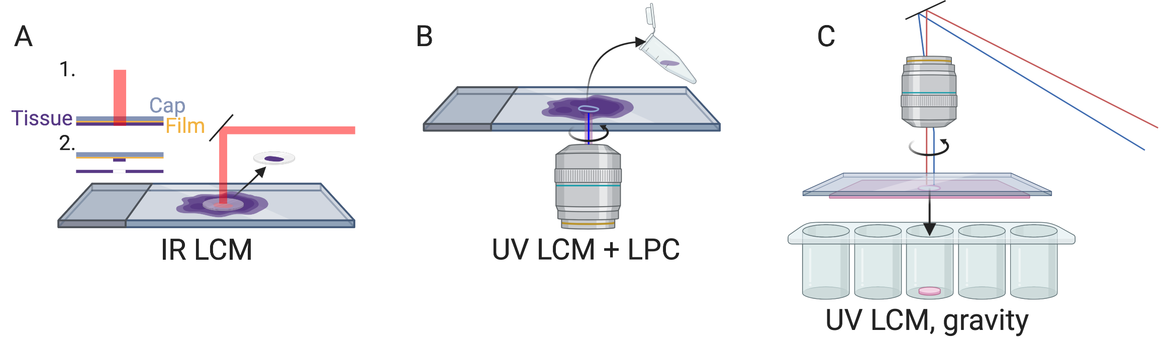
A) IR LCM schematic. B) UV LCM and LPC schematic, like in Zeiss PALM Microbeam. C) UV LCM, letting microdissected region fall by gravity, like in Leica LMD. All schematics in this book, i.e. anything not made with ggplot2, were created with BioRender.com

Figure 5.1: A) IR LCM schematic. B) UV LCM and LPC schematic, like in Zeiss PALM Microbeam. C) UV LCM, letting microdissected region fall by gravity, like in Leica LMD. All schematics in this book, i.e. anything not made with ggplot2, were created with BioRender.com

At present, there are two main types of LCM: IR and UV. IR LCM was introduced in 1996 (Emmert-Buck et al. 1996). It utilizes a cap with thermoplastic film which is placed over an area of interest, and an IR laser to briefly heat select areas of tissues to 90 °C so the film melts in the area and fuses to the area of tissue of interest (Emmert-Buck et al. 1996) (Figure 5.1 A). This was commercialized as the Arcturus PixCell II LCM System in 1997, which was used in several early LCM studies including the first one in 1999 (Luo et al. 1999; Ohyama et al. 2000; Sgroi et al. 1999; Kitahara et al. 2001) (Figure 4.3).

UV LCM is also known as laser microbeam microdissection (LMM) due to the microbeam of UV laser used. A popular commercial UV LCM system is the Robot-Microbeam (P.A.L.M. Wolfratshausen, Germany), now Zeiss PALM Microbeam. In this method, a narrow UV laser beam ablates a narrow strip of tissue surrounding the area of interest, isolating the area of interest from the rest of the section, so the area of interest is minimally heated. Then, the area of interest is removed from the slide into the collection vial with laser pressure catapult (LPC), avoiding physical contact so as to prevent cross contamination (Figure 5.1 B). An early version of this system was first used in 1996 to isolate single cells from gastric tumors, followed by PCR to analyze E-cadherin mutations, but the cells were removed with a needle rather than LPC (Becker et al. 1996). Another popular commercial UV LCM system is the Leica LMD; unlike the PALM system, the Leica system lets the isolated tissue fall into collection vials by gravity, still avoiding physical contact (Figure 5.1 C). UV LCM was used in some early LCM spatial transcriptomics studies as well (Nakamura et al. 2004), and remains popular in recent years while IR LCM seems to have fallen out of favor (Moor et al. 2017; Zechel et al. 2014; Baccin et al. 2020).

Recent versions of the Arcturus LCM system have both IR and UV, which can be used in conjunction. UV can be used to cut the region of interest (ROI) and IR can then be used to fuse the region to the film at a few points for removal (“Arcturus XT Laser Capture Microdissection (LCM) Instrument - US,” n.d.).

5.1.1.2 Amplification

The minuscule amount of transcripts from microdissected tissues, which can be single cells, needs to be amplified to be detected by microarray or RNA-seq. Indeed, RNA amplification is a part of one of the most prevalent topics in LCM related search results (Figures 6.3, 6.4). To this day, there are two main strategies of amplification of minuscule amount of mRNA or cDNA – in vitro transcription (IVT) of cDNA (linear amplification) and PCR (exponential amplification), or a combination of both (Tang, Lao, and Surani 2011). These two strategies have coexisted since their beginnings in 1989 and 1990 (Figure 4.3).

Heterogeneous cDNAs can be amplified with PCR by appending known sequences to one or both ends of the cDNA so primers with known sequences can be used to amplify the heterogeneous cDNAs. Early approaches meant for single cells or small number of cells include tailing the cDNA with poly-dA (Belyavsky, Vinogradova, and Rajewsky 1989) or poly-dG (G. Brady, Barbara, and Iscove 1990) after reverse transcription, and use as PCR primers sequences containing poly-dT (both poly-dA tail and reverse transcription (RT) primer of poly-A mRNAs) or poly-dC (poly-dG tail) and poly-dT (RT primer). Alternatively, lone linkers (“lone” because they are designed to prevent linker polymerization) could be ligated to both ends of the DNA fragments of interest to anneal to PCR primers (M. S. H. Ko et al. 1990). Some of the early single cell (or small number of cells) transcriptomic studies used PCR amplification, prior to quantification or differential expression analyses with Southern blot with radiolabeled cDNA probes hybridizing to cDNA clones of interest screened from plaque lift hybridization of a phage cDNA library (Dulac and Axel 1995), or with cDNA microarray (C. A. Klein et al. 2002; Tietjen et al. 2003). LCM was used to isolate the single cells in (Tietjen et al. 2003). Before the advent of CEL-seq, early scRNA-seq methods also used PCR amplification (Tang et al. 2009; Islam et al. 2011). An influential method is switching mechanism at the 5′ end of the RNA transcript (SMART) (Y. Y. Zhu et al. 2001), for construction of cDNA (clone) libraries covering the full length of mRNAs, though not originally for single cells. The full length scRNA-seq method Smart-seq(2) (Ramsköld et al. 2012) is based on SMART but adapted to the minuscule amount of transcripts from single cells, with PCR amplification of the cDNA. Smart-seq(2) is one of the most commonly used library preparation methods for LCM since the 2010s, and was used for RNA-seq of LCM isolated single cells (Nichterwitz et al. 2016).

Alternatively, transcripts can be amplified by IVT, with a T7 RNA polymerase promoter attached to the 5’ end of the poly-dT primer, so the RNA polymerase transcribes the cDNAs into many copies of antisense RNAs (aRNA) (Gelder et al. 1990; Eberwine et al. 1992). Some of the early single cell (or small number of cells) transcriptomic studies used IVT amplification. Quantification and differential expression analyses of the aRNA can be performed with differential display (Liang and Pardee 1992; Kacharmina, Crino, and Methods in Enzymology Eberwine 1999), cDNA microarray (Hemby et al. 2002; Kamme et al. 2003), or with “expression profiling” (Eberwine et al. 1992; Kacharmina, Crino, and Methods in Enzymology Eberwine 1999), i.e. reverse northern blot with radiolabeled aRNAs hybridizing to cDNA clones of interest, where the cDNA clones can be blotted onto a Southern blot membrane in a macroarray, which may have inspired the development of the cDNA microarray printed on glass (Kacharmina, Crino, and Methods in Enzymology Eberwine 1999). LCM was used to isolate the single cells in (Kamme et al. 2003). Since the 2010s, Cell Expression by Linear amplification and Sequencing (CEL-seq) (Hashimshony et al. 2012) and derivatives (e.g. CEL-seq2, MARS-seq, and SORT-seq), which use IVT amplification, have been commonly used for library preparation for microdissected or de facto microdissected samples such as from LCM (Tzur et al. 2018), Tomo-seq (Junker et al. 2014), and Niche-seq (Medaglia et al. 2017).

5.1.2 Usage of LCM

Usage trends of LCM as reflected in PubMed and bioRxiv search results are analyzed in Chapter 6. LCM can be used to isolate targeted ROIs based on histology, or to create a grid for untargeted search of gene expression patterns in space, and examples of both are highlighted here. Moreover, the three themes of screening, atlas curation, and new technique development, are all represented in LCM literature. In the “screening” theme, LCM is used to isolate cell populations of interest based on histology (targeted) to discover genes associated with pathological conditions such as cancer metastasis (Nakamura et al. 2004) and cell types (Aguila et al. 2018), or to discover cell type localization in healthy tissue difficult to other spatial transcriptomics techniques such as the bone marrow (Baccin et al. 2020).

LCM can also be used to dissect the tissue in a grid, not targeting very specific histological regions (untargeted), to identify genes associated with locations on the grid (Moor et al. 2018; G. Peng et al. 2016) or transcriptomically defined regions (Zechel et al. 2014; G. Peng et al. 2016), or to map cells from scRNA-seq to spatial locations (Zechel et al. 2014; G. Peng et al. 2016). The untargeted studies can also touch upon the “atlas” theme, providing an online interface to query and explore the spatial transcriptomes (G. Peng et al. 2016).

However, targeted approaches can also be used for the “atlas” theme, such as in the human (Hawrylycz et al. 2012; J. A. Miller et al. 2014) and macaque (Bakken et al. 2016) atlases of the ABA, isolating histologically annotated regions for microarray profiling to build systematic resources for exploration. This addresses the limitation of bright field ISH that only one gene can be stained per section thus requiring large number of brains, which is too costly for primates; in LCM, while often not single cell resolution, the same brain can be used to profile the whole transcriptome. The “technique development” theme is evident in the text mining results (Figure 6.3), and contributes to some of the advantages of LCM as discussed below.

As shown in Chapter 6, LCM transcriptomics has spread far and wide, and has been used on many research topics rarely featured in (WM)ISH atlases. These include cancer and botany (Figure 6.2, Figure 6.3). The following advantages of LCM might have contributed to its popularization: first, as already mentioned, both IR and UV LCM systems have been commercialized prior to their use for transcriptomics, making setup convenient. Second, while LCM equipment can be expensive and require specialized training to use, many institutions have core facilities that can perform LCM (“Translational Pathology Core Laboratory (TPCL),” n.d.; “Veritas Laser Capture Microdissection (LCM) and Laser Cutting System from Applied Biosystems,” n.d.; “Dana-Farber Core Facilities,” n.d.; “Johns Hopkins Cell Imaging Core Facility,” n.d.), reducing cost and personnel training time in individual laboratories.

Third, in some cases, especially in the clinical setting, only archival formalin fixed, paraffin embedded (FFPE) tissues are available. While in 2020, newer current era technologies such as Visium (Villacampa et al. 2020) and GeoMX DSP (Hwang et al. 2020) have been demonstrated on FFPE tissues, LCM followed by microarray was already demonstrated on FFPE tissues in 2007 (Coudry et al. 2007) and with RNA-seq by 2014 (Morton et al. 2014). As a result, for several years, LCM may have been the only option to perform spatial transcriptomics on FFPE samples. In addition, LCM might still be the only way to profile transcriptomes of single cells in FFPE samples. With scRNA-seq library preparation methods such as Smart-seq2 (Nichterwitz et al. 2016), and CEL-seq (Tzur et al. 2018) it is possible to profile the transcriptome in minuscule amount of LCM isolated tissue, and even single cells (Nichterwitz et al. 2016). With Smart-3SEQ, LCM single cell transcriptomics has been made possible for FFPE tissues as well, even for samples that are several years old (Foley et al. 2019).

Finally, despite its long history, LCM cannot yet be replaced by newer spatial transcriptomics technologies. Unlike smFISH or ISS based techniques, LCM followed by RNA-seq is not restricted to known genes and allows for transcriptome wide profiling and other omics. Unlike ST and Visium, LCM can have single cell resolution, and unlike array based techniques with resolution of the size of a cell or higher, such as Slide-seq(2) and HDST, LCM can more unequivocally isolate individual cells or nuclei based on histology.

LCM has a number of disadvantages, some of which are addressed by other current era spatial transcriptomics technologies. First, compared to droplet based scRNA-seq and highly multiplexed barcoding, using LCM to isolate single cells is still too laborious, limiting its throughput. Second, LCM requires tissue sections, while preparation of many slides to cover a 3D volume can be laborious and it can be challenging to reconstruct 3D structures from tissue sections. To reiterate, sections of blastoderm stage embryos are hard to interpret, which motivated WMISH. Third, because it can be challenging to segment cells based on hematoxylin and eosin (H&E) or immunohistochemistry (IHC) staining and parts of different cells can be stacked within the thickness of the section even in thin sections, single cells isolated by LCM can have contents of other cells.

5.1.3 Physical microdissection

5.1.3.1 Voxelation

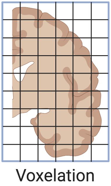
Figure 5.2: Voxelation of human brain, as in (Vanessa M. Brown 2002).

LCM did not completely replace microdissection with a physical blade. Voxelation was one of the alternatives to LCM developed to profile spatial transcriptomes in 3D and address the limitation of throughput of ISH. In voxelation, a grid of steel blades is used to cut tissue into cubes for microarray profiling, but the resolution is low. Human brains were first cut into 8 mm thick slabs and then a grid of 1 cm per side (Vanessa M. Brown 2002; Singh et al. 2003), and mouse brains were first cut into 1 mm thick slabs and then a grid of 1 mm per side (V. M. Brown et al. 2002; Singh et al. 2003; Chin et al. 2007) (Figure 5.2). With low resolution, it’s easier to use voxelation to profile large 3D tissues of multiple slabs that would be much more laborious with LCM’s thinner sections and higher resolution (V. M. Brown et al. 2002). As the human voxels were quite large (almost 1 ml) and corresponding voxels of 20 to 30 mice were pooled (V. M. Brown et al. 2002; Chin et al. 2007) to get enough transcripts, the voxelation studies did not mention T7-based PCR amplification of transcripts, unlike for LCM samples (Nakamura et al. 2004). To the best of our knowledge, voxelation never spread beyond its institution of origin, UCLA School of Medicine, and has not been used in a publication to generate new data since 2007 (Chin et al. 2007) and for data analysis since 2009 (An et al. 2009).

5.1.3.2 Tomo-seq

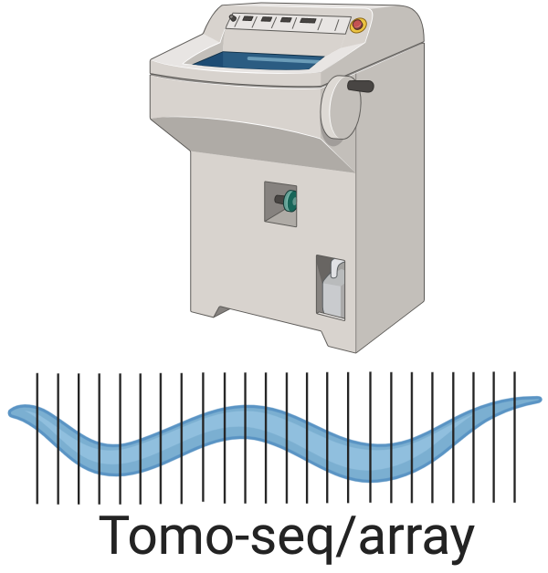
Figure 5.3: Tomo-seq, here showing C. elegans.

Another alternative to LCM is Tomo-seq/array, which has continued to be utilized in recent years. In this approach, the tissue is sectioned with a cryotome like tomography (hence the “Tomo”), and the transcripts in each section are extracted for microarray (Tomo-array) or RNA-seq (Tomo-seq) profiling; the resolution is limited by section thickness, which has gone down to 8 \(\mu\)m (Brink et al. 2020). Three-D expression maps can be reconstructed from sections along the anterior-posterior (AP), dorsal-ventral (DV), and left-right (LR) axes. All three themes, namely screening, atlas curation, and new technique development, are present in Tomo-seq/array literature.

Tomo-array was first used in 2012 to build a 3D mouse brain transcriptome atlas, attempting to address difficulties in image registration in ISH atlases, low resolution of voxelation, and limitation of LCM to specific regions (Okamura-Oho et al. 2012) (Figure 4.3). Mouse brains were sectioned along all three axes and 200 adjacent 5 \(\mu\)m sections were pooled as “fractions” for microarray; again, PCR amplification was not mentioned. Fractions from the three axes were then used to reconstruct a 3D atlas.

Tomo-seq was first demonstrated in 2013, on Drosophila melanogaster embryos, with 60 and 25 \(\mu\)m sections, again in response to the difficulty to scale ISH atlases to the whole transcriptome (Combs and Eisen 2013). Genes patterned along the AP axis were identified, and the data is stored in an online database. However, Tomo-seq is more commonly credited to a 2014 method first demonstrated on zebrafish embryos, with 18 \(\mu\)m sections (Junker et al. 2014). Gene expression patterns along the AP axis of straightened embryos were identified, and sections along all three axes were used for 3D reconstruction of embryos that were not straightened. The data and the 3D reconstruction are also stored in an online database, though the 3D reconstruction algorithm produced many artefacts.

Since then, Tomo-seq has been used in several different biological systems, typically when one axis is of primary interest. Tomo-seq has been used in C. elegans (Ebbing et al. 2018), developing zebrafish hearts (Burkhard and Bakkers 2018), Drosophila embryos (Combs and Fraser 2018), ischemic mouse hearts (Lacraz et al. 2017), and Pristionchus pacificus (Rödelsperger et al. 2020) to identify genes associated with that axis of interest. Tomo-seq was also used on mouse (Brink et al. 2020) and human (Moris et al. 2020) gastruloids to demonstrate the viability of this in vitro and potentially high-throughput model for developmental biology. Again, due to the minuscule amount of tissue in each section, library preparation methods designed for scRNA-seq, such as CEL-seq(2) (Junker et al. 2014; Rödelsperger et al. 2020; Ebbing et al. 2018) have been adapted to Tomo-seq.

5.1.3.3 Other methods of physical microdissection

Algorithms inspired by reconstruction of ray-based computerized tomography have been used to reconstruct spatial patterns of gene expression from Tomo-seq-like slices cut from different angles of the same tissue with a stereotypical structure. This was first attempted with Gene Expression Tomography (GET) (Vanessa M. Brown et al. 2002), though only on qPCR quantification of one gene in those slices. More recently, this kind of idea was used in Spatial Transcriptomics by Reoriented Projections and sequencing (STRP-seq), in response to the limited number of genes of smFISH and ISS based techniques, degradation of RNA and technical complexity of LCM, and number of specimens required by and inadequacy of the 2014 Tomo-seq 3D reconstruction (Schede et al. 2020). This has been shown to perform better than the 2014 Tomo-seq 3D reconstruction method, and was demonstrated on the brain of a non-model organism, the lizard Pogona vitticeps.

Because of the specialized equipment and technical complexity of LCM and degradation of RNA, other methods of physical microdissection have been developed. Examples of such techniques are Cell and Tissue Acquisition System (CTAS), which uses a disposable capillary unit connect to the vacuum to aspirate tissue (Kudo et al. 2012), and an automated micropuncch system that collects samples of tissue with diameter of 110 \(\mu\)m at 300 \(\mu\)m intervals (Yoda et al. 2017). In addition, for similar reasons, manual microdissection is still used (Figure 4.7), such as to dissect leaves on a grid of distances from a lesion to characterize response to infection (Giolai et al. 2019; Lukan et al. 2020). Manual microdissection of pre-defined anatomical regions was also used to create low resolution gene expression atlases of Xenopus laevis (Plouhinec et al. 2017) and Xenopus tropicalis (Blitz et al. 2017) embryos, to avoid sectioning as required for LCM and artefacts in Tomo-seq 3D reconstruction.

5.1.4 De facto microdissection

Some methods have been developed that do not directly cut tissues. Instead, cells, or ROIs judged from histology, are optically and molecularly marked so that only transcripts or cells from the marked regions are captured. Because these methods involve selection of pre-defined ROIs within the section, we call them de facto microdissection.

Transcriptome in vivo analysis (TIVA) from 2014 can be viewed as the first of these methods (Lovatt et al. 2014). Live cell culture is incubated with the photoactivable cage with a poly-U sequence that captures poly-A transcripts. Select cells are photoactivated by 405 nm laser and the captured transcripts are sequenced. TIVA is widely cited, perhaps because it is one of the earliest single cell resolution and transcriptome wide methods, predating RNA-seq from LCM isolated single cells. However, because TIVA has only been demonstrated on fewer than a dozen cells per sample, to the best of our knowledge it has not been used in any other publication to collect new data.

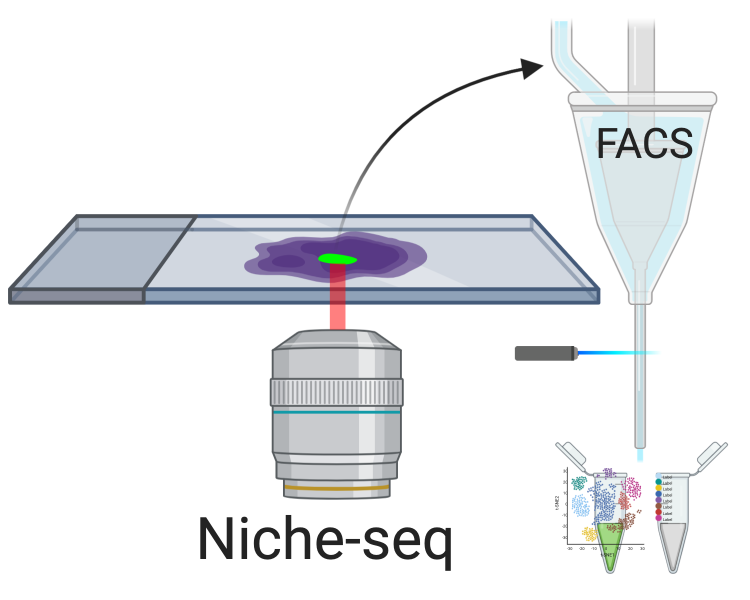
Figure 5.4: Niche-seq schematics. Green: cells with photoactivated PA-GFP.

A de facto microdissection method that has spread beyond its institution of origin is Niche-seq, which was developed as LCM is still usually used to isolate groups of cells rather than single cells and involves tissue fixation (Medaglia et al. 2017). Select regions of ex vivo tissues from transgenic mice expressing photoactivable GFP (PA-GFP), here lymph node and spleen B cell and T cell niches, are photoactivated at 820 nm with two photon irradiation. Then the tissue is dissociated and cells with photoactivated PA-GFP are collected from flow cytometry-based fluorescence-activated cell sorting (FACS) for scRNA-seq with MARS-seq (Figure 5.4). This approach was originally used in 2010 to isolate B cells from light and dark zones of the lymph node followed by transcriptome profiling with microarray in bulk (Victora et al. 2010); the difference in Niche-seq is scRNA-seq of the sorted cells. After its inception, Niche-seq has been used once more in lymph node niches (Giovanni et al. 2020). However, as Niche-seq requires transgenic mice expressing PA-GFP and living tissue, it cannot be applied to human tissues, to fixed tissues, or when a PA-GFP line is unavailable. This might limit further growth of Niche-seq. Moreover, the spatial context of cells within the photoactivated region is lost, limiting spatial resolution.

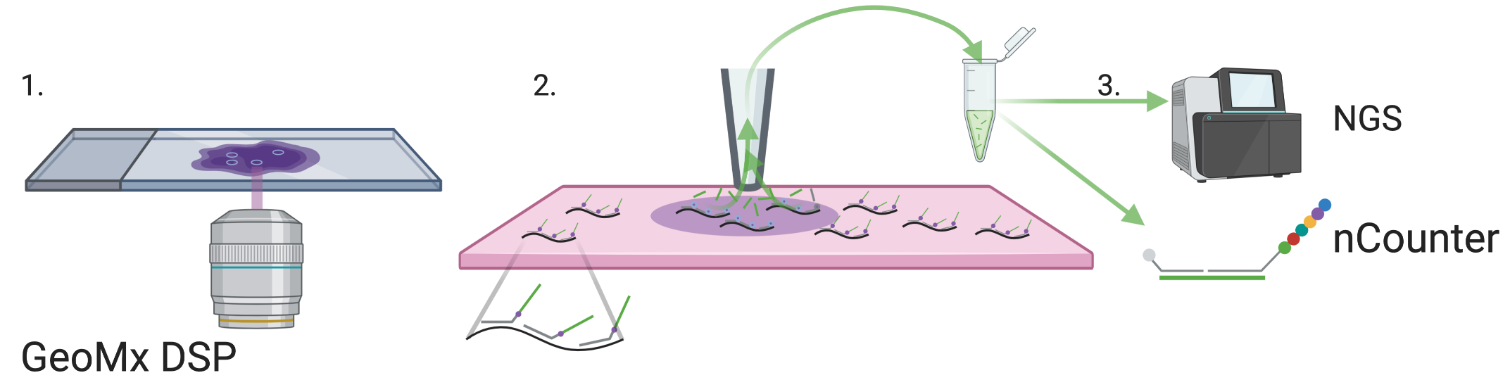
Figure 5.5: GeoMX DSP schematics, inspired by figures in (Merritt et al. 2020). Black: transcripts in tissue. Gray: probes. Green: indexing oligo.

Another method that spread beyond its institution of origin is the commercial GeoMX DSP from NanoString (Merritt et al. 2020), which can be used for both high throughput immunofluorescence and transcript quantification in FFPE tissue sections. While GeoMX DSP does not physically isolate relevant parts of the tissue, it is discussed in this section because like other microdissection based techniques, GeoMX DSP is primarily ROI based, and spatial location is known from selection of the ROI. For transcript quantification, probes are attached to indexing oligos with a UV cleavable linker (Figure 5.5). The selected ROI is illuminated by UV to remove the index oligos from the probes. Then the released index oligos are aspirated and quantified with either NGS or NanoString nCounter. This can be repeated for multiple ROIs, which can be a grid for unbiased profiling (Merritt et al. 2020). The probes tile the transcripts, and each probe has a distinct index oligo, so in NGS, each tile is counted separately, enabling isoform quantification (Merritt et al. 2020). The number of genes profiled by GeoMx DSP depends on the gene panel used; the Cancer Transcriptome Atlas panel with over 1800 genes have been used in several studies (e.g. (Margaroli et al. 2021; Jiwoon Park et al. 2021)), and with the human or mouse Whole Transcriptome Atlas (WTA) panel, transcripts of 18190 genes can be quantified, nearly covering the whole transcriptome (K. Roberts et al. 2021). In GeoMX WTA, the UV cleaved index oligo must be sequenced with NGS to identify the gene each transcript is from. As pre-defined probes are required, unlike in RNA-seq, novel transcripts cannot be quantified. Ready made probe sets for oncology, immunology, and neuroscience are sold by NanoString (“Gene Expression Panels | NanoString Technologies,” n.d.). Although GeoMx DSP was published in 2019, it has spread to several different institutions, and has been used on pancreatic ductal adenocarcinoma (PDAC) (Hwang et al. 2020), hepatocellular carcinoma (HCC) (Ankur Sharma et al. 2020), reactive lymph nodes (Tripodo et al. 2020), and COVID infected lungs from autopsy (Jiwoon Park et al. 2021; Butler et al. 2021; Delorey et al. 2021; Margaroli et al. 2021).

5.1.5 Targeted vs. untargeted

Some methods can only be used in a regular grid, such as Tomo-seq, while some can be used either in a regular grid or in targeted ROIs, such as LCM and GeoMX DSP (Figure 5.6. Some are primarily used for targeted ROIs, such as Niche-seq. Sometimes an= targeted ROI in the section may be chosen, which is then divided into smaller regular parts, in between targeted and untargeted.

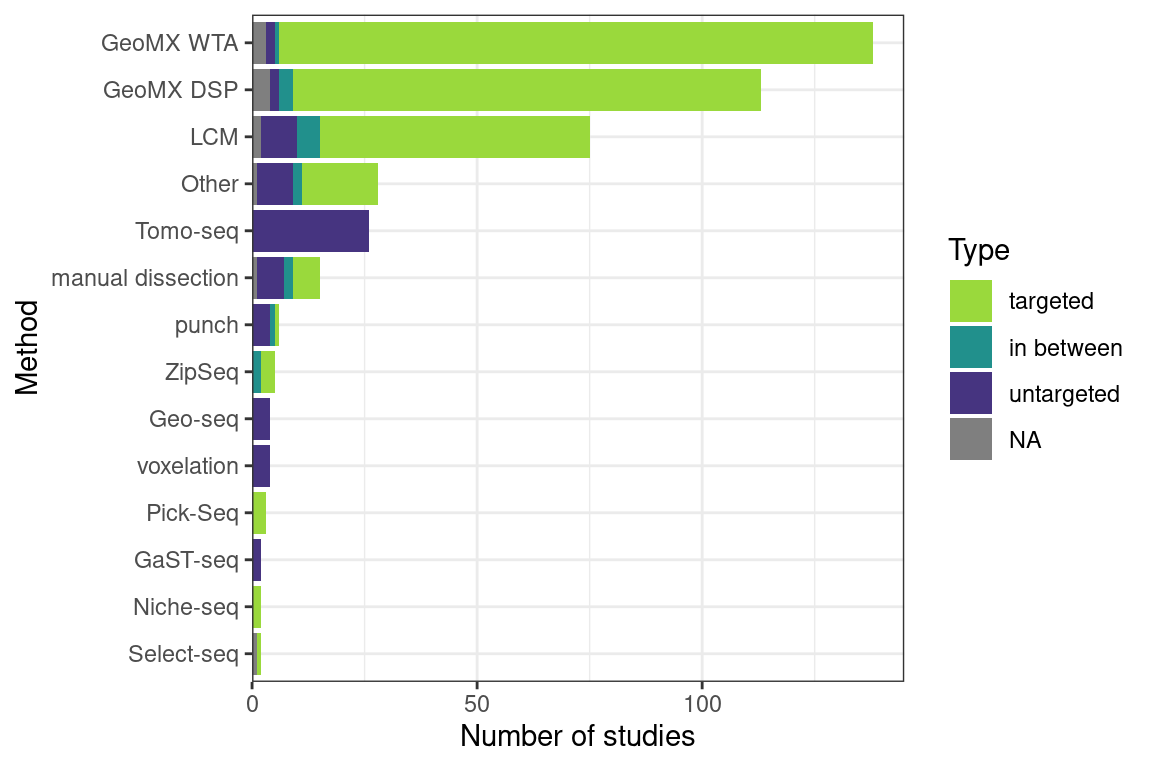
Number of studies of each of the three types: targeted, in between, and untargeted, using each microdissection based technique plus GeoMX DSP. Techniques used in less than two studies or two types are lumped into Other.

Figure 5.6: Number of studies of each of the three types: targeted, in between, and untargeted, using each microdissection based technique plus GeoMX DSP. Techniques used in less than two studies or two types are lumped into Other.

After LCM, GeoMX DSP/WTA is the most popular targeted ROI based technique, and as already mentioned, GeoMX DSP has been used in several COVID autopsy studies. GeoMX DSP is often used to profile proteins, which is beyond the scope of this book; our database only contains metadata for GeoMX DSP transcriptomic datasets. As of writing, all GeoMX DSP datasets in our database are from human, and are from predominantly pathological FFPE tissues (Figures 5.7, 5.8). Because of COVID, GeoMX DSP is more used on the lungs for transcriptomics than other tissues (Figure 5.9).

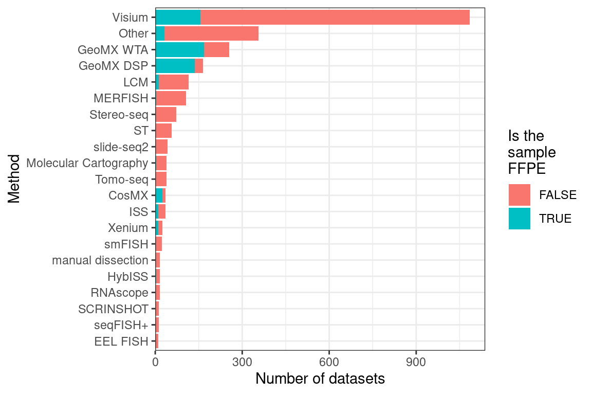
Number of FFPE and frozen section datasets from each current era technique; techniques used in fewer than 10 datasets are lumped into Other. LCM is only for curated LCM literature and does not include all search results in Chapter 6.

Figure 5.7: Number of FFPE and frozen section datasets from each current era technique; techniques used in fewer than 10 datasets are lumped into Other. LCM is only for curated LCM literature and does not include all search results in Chapter 6.

Number of FFPE and frozen section datasets from each current era technique in humans and mice healthy and pathological tissues; techniques used in fewer than 10 datasets are lumped into Other. LCM is only for curated LCM literature and does not include all search results in Chapter 6.

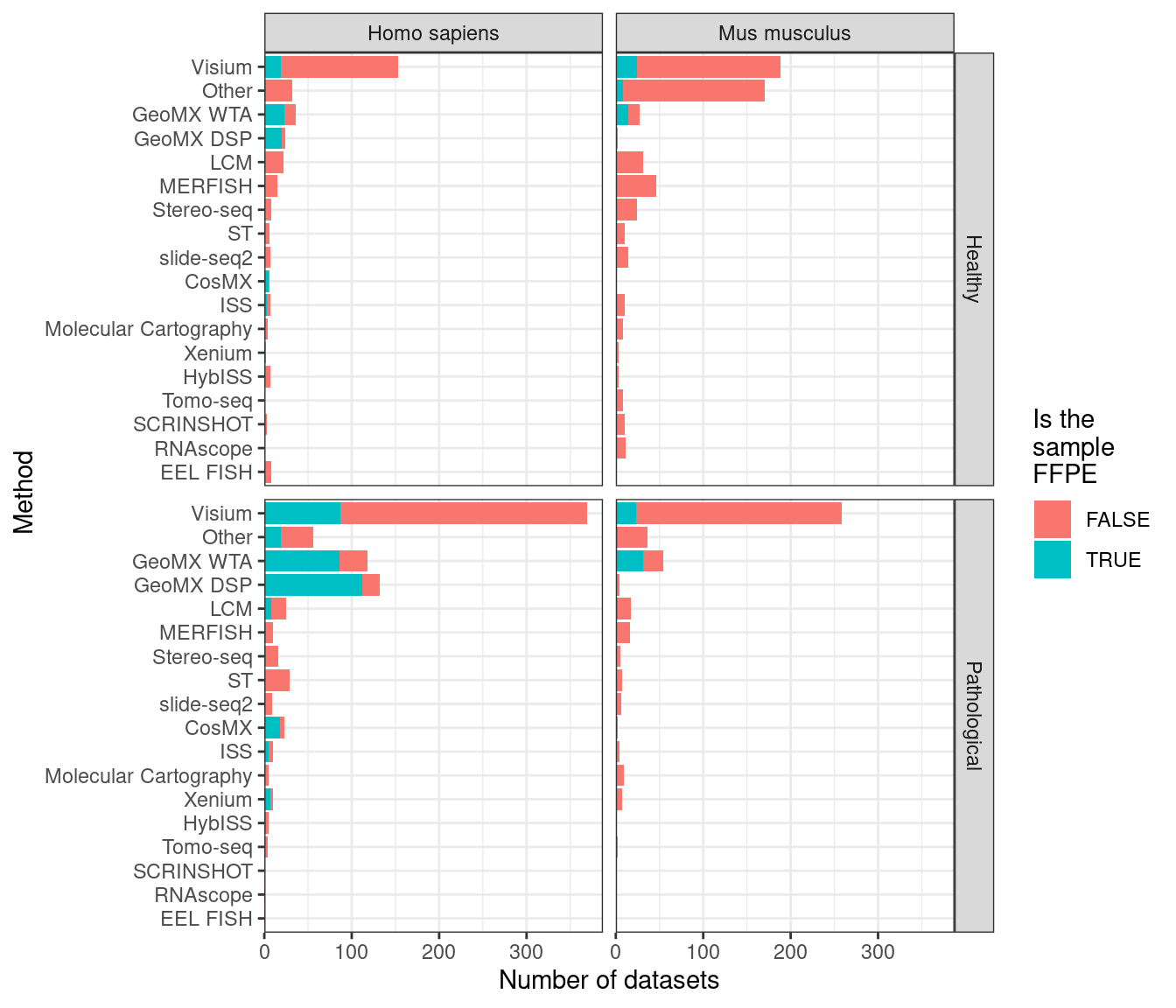
Figure 5.8: Number of FFPE and frozen section datasets from each current era technique in humans and mice healthy and pathological tissues; techniques used in fewer than 10 datasets are lumped into Other. LCM is only for curated LCM literature and does not include all search results in Chapter 6.

Number of GeoMX DSP or WTA studies for healthy and pathological human organs. Male is shown here because there are studies for the prostate but not for female specific organs.

Figure 5.9: Number of GeoMX DSP or WTA studies for healthy and pathological human organs. Male is shown here because there are studies for the prostate but not for female specific organs.

In an earlier version of this book, in the current era, ROI selection (formerly Microdissection) was the most widely used type of techniques. However, NGS barcoding has surpassed ROI selection more recently due to the rapid growth of popularity of Visium (Figure 5.10). Excluding LCM, GeoMX DSP and Tomo-seq are the most popular techniques after ST and Visium (Figure 4.7). ROI selection has not been replaced by other seemingly more sophisticated techniques such as ST and MERFISH, and is still popular in 2020 and 2021 (Figure 4.1, Figure 6.1). ROI selection techniques generally do not have single cell resolution, but combined with scRNA-seq or snRNA-seq data, cell type compositions of ROIs can be computationally deconvoluted (Baccin et al. 2020; Hwang et al. 2020). The popularity may be due to availability of commercial platforms (LCM and GeoMX DSP), core facilities (LCM, NGS, and Nanostring nCounter for GeoMX DSP), Nanostring’s Technology Access Platform (TAP), a commercial data collection and analysis service for GeoMX DSP (“DSP Technology Access Program (TAP),” n.d.), not requiring specialized equipment (Tomo-seq, manual microdissection), or disadvantages of other techniques discussed later in this chapter.

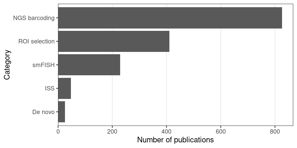
Figure 5.10: Number of publications per category of techniques in the current era. Non-curated LCM literature is excluded.

5.2 Single molecular FISH

One quantitative approach to transcript abundance estimation is to display individual transcripts as distinct puncta with FISH and count them. Prior to smFISH, transmission electron microscopy was used to visualize individual mRNA molecules in fibroblasts by labeling the poly-A tail with a single large colloidal gold particle and the in situ reverse transcribed cDNA with small gold particles (Bassell et al. 1994). That FISH can be used to visualize single mRNA molecules was first demonstrated in 1998 (Femino et al. 1998) (Figure 4.3). Five or more probes targeting adjacent parts of the transcript, each about 50 nt long and labeled with 5 fluorophores were hybridized to the transcripts. The puncta seen were shown to be likely individual mRNA molecules, as the fluorescence intensity of each punctum was consistent with the number of fluorophores, and the number of puncta for \(\beta\)-actin was consistent with the number of \(\beta\)-actin transcripts measured by other means, and the colors of puncta seen from probes with different colored fluorophores targeting different parts of the transcript were consistent with organization of the fluorophores on the transcript (Figure 5.11).

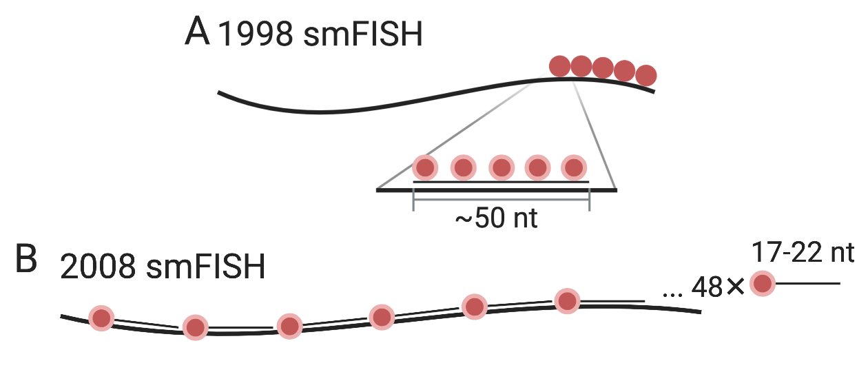
A) Schematic of smFISH from (Femino et al. 1998). The long thick line stands for the mRNA, and short think line stands for DNA oligo probe. B) smFISH with singly labeled probes from (Raj et al. 2008).

Figure 5.11: A) Schematic of smFISH from (Femino et al. 1998). The long thick line stands for the mRNA, and short think line stands for DNA oligo probe. B) smFISH with singly labeled probes from (Raj et al. 2008).

The 1998 approach had a number of disadvantages, leading to development of an alternative approach in 2008 (Raj et al. 2008). First, probes labeled with multiple fluorophore moieties are difficult to synthesize and purify. Second, the multiple fluorophores on the same probe can interact with each other and self-quench. Third, out of the 5 probes per transcript, only 1 or 2 may have actually hybridized to the transcript in most cases, making it difficult to distinguish between true signal and non-specific binding. In the 2008 method, each 17-22 nt probe is labeled with one fluorophore at the 3’ end, and a larger number of probes (48 or more) targeting tandem sequences of the transcript were used to improve signal to noise ratio (Figure 5.11). The probes were computationally designed and ordered from Biosearch Technologies. This method influenced later highly multiplexed smFISH techniques; computational probe design and commercial synthesis would remain crucial.

5.2.1 Barcoding strategies

To use smFISH to quantify transcripts transcriptome wide, there is an obvious challenge – how to distinguish among over 20,000 genes with only about 5 easily distinguishable colors? Various strategies using multiple colors and/or rounds of hybridization or imaging have been devised to drastically expand the palette. The first attempt to do so was in 1989, using 3 colors to visualize 4 chromosomes in immunological DNA FISH (Nederlof et al. 1990) (Figure 4.3). Each probe can be labeled with one or two of the 3 haptens: biotin, 2-acetyl aminofluorene (AAF), and Chemiprobe. Red fluorophore was attached to avidin to target biotin label, and blue and green to different secondary antibodies targeting, respectively, mouse anti-Chemiprobe and rabbit anti-AAF primary antibodies (Figure 5.12). Then with one doubly labeled and 3 singly labeled probes, imaged with different excitation wavelengths or channels, 3 colors can distinguish 4 chromosomes. However, with this method, the palette size is limited by the number of haptens available and the number of their combinations.

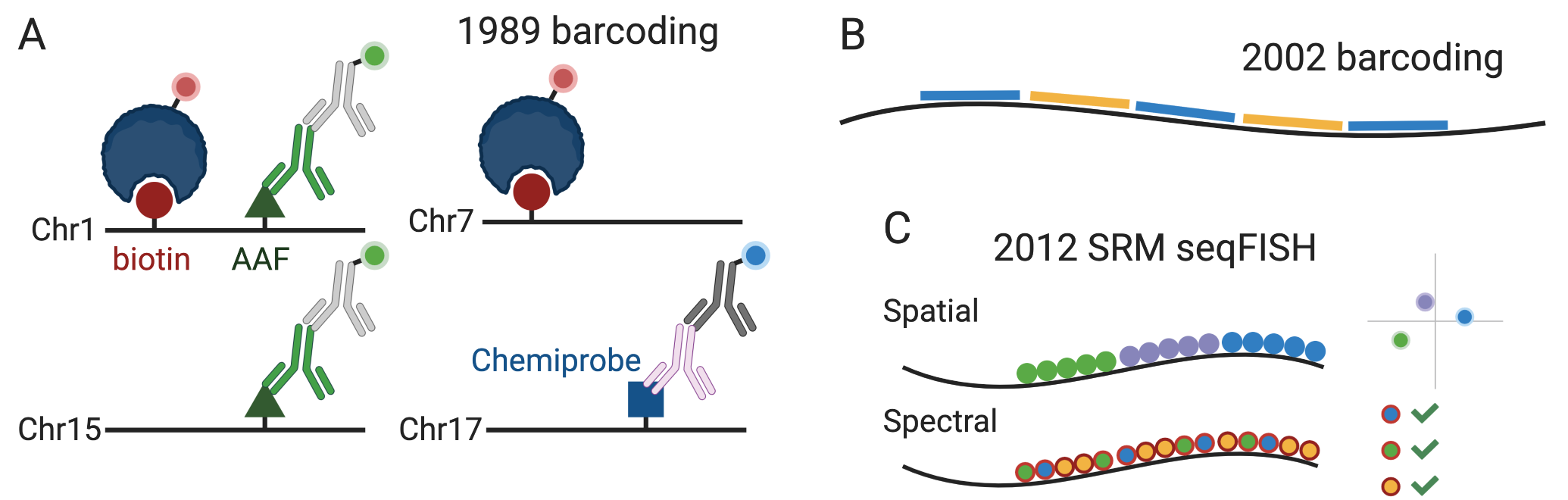
A) Combinatorial barcoding in immunological DNA FISH, as described in (Nederlof et al. 1990). The line stands for the probe and the circle, triangle, and square stand for haptens. Not to scale, and only one hapten of each kind is shown on one probe. B) Combinatorial barcoding in (Levsky 2002). Short colored lines stand for probes with fluorophores of the color. C) Schematic of SRM seqFISH as described in (Lubeck and Cai 2012).

Figure 5.12: A) Combinatorial barcoding in immunological DNA FISH, as described in (Nederlof et al. 1990). The line stands for the probe and the circle, triangle, and square stand for haptens. Not to scale, and only one hapten of each kind is shown on one probe. B) Combinatorial barcoding in (Levsky 2002). Short colored lines stand for probes with fluorophores of the color. C) Schematic of SRM seqFISH as described in (Lubeck and Cai 2012).

For transcript detection, to our best knowledge, the first attempt was in 2002 (Levsky 2002); fluorophore labeled probes were synthesized as in the 1998 smFISH method, and either probes of one color or a mixture of probes of 2 colors were hybridized to the transcript, and imaged with different channels, to visualize transcription foci in the nucleus (Figure 5.12). This way, combinations of 2 of the 4 available colors plus blank were used to encode 10 different transcripts.

The above mentioned historical works in smFISH and combinatorial barcoding laid foundation to smFISH based spatial transcriptomics. The first attempt to quantify transcripts with combinatorial barcoding at single molecular resolution was in 2012 by Long Cai’s group, which later developed seqFISH and its variants (Lubeck and Cai 2012). Like in the 2008 smFISH study, singly labeled probes purchased from Biosearch were used, but forming blocks of different colors as in the 1998 smFISH \(\beta\)-actin experiment. Then the transcripts were imaged with super-resolution microscopy (SRM), in particular stochastic optical reconstruction microscopy (STORM). In the spatial barcoding strategy, the ordering of the colors in space would distinguish between transcripts, but would require linearization of the transcripts and high resolution (20 nm) (Figure 5.12). To improve signal to noise ratio, cyanine dye–based photoswitchable dye pairs (Bates et al. 2012) was used so both the activator and the emitter fluorophores must be present and adjacent for the fluorophores to be reactivated. In the spectral barcoding approach, the pairs of fluorophores are spread across the transcript, so the transcripts are recognized by the pairs of fluorophores detected (Figure 5.12). The spectral approach requires lower resolution (100 nm) and does not require linearization, but because the ordering of the colors is not used, the number of possible barcode from the same number of colors is smaller than in the spatial approach. With spectral barcoding, transcripts of 32 genes were quantified in yeast, with 3 color barcodes chosen from 7 available colors. To the best of our knowledge, after its inception, this SRM method has not been used to generate new data, perhaps because it requires specialized equipment for SRM. None of the later methods in our curated database used SRM.

Thus far, probes with fluorophores of different colors were hybridized to mRNAs at the same time, without multiple rounds of hybridization. To obtain single molecular resolution but without SRM, there is a challenge of needing to use multiple probes of the same color to strengthen signal, which requires transcripts that are long enough to accommodate probes of different colors. The more colors that are used to encode more genes, the longer the transcripts must be.

This changed in 2014, with the advent of seqFISH (Lubeck et al. 2014). Twenty four singly labeled probes were designed for each gene, and 12 genes were encoded with 4 colors and 2 rounds of hybridization (Figure 5.13). After imaging the first round of hybridization and DAPI staining for DNA, the probes are removed with DNase I, and then probes for the second round are hybridized. Let \(F\) denote the number of fluorophores or colors, and \(N\) denote the number of rounds of hybridization, then the number of genes that can be barcoded is \(F^N\). However, with longer barcodes to encode more genes, error can build up.

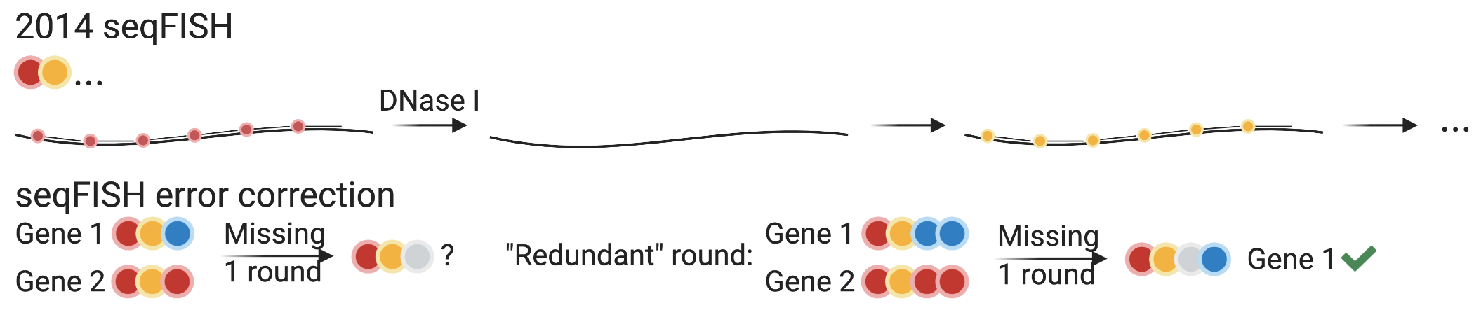
Figure 5.13: Probe structures of 2014 seqFISH (Lubeck et al. 2014) and seqFISH error correction.

The most common error in multi-round smFISH is missing signal, most likely in one round (Shah et al. 2016; K. H. Chen et al. 2015). If all \(F^N\) barcodes are used and one round is missing for a mRNA molecule, then the existing signal of this molecule is consistent to \(F\) genes, so it cannot be uniquely identified. If a small proportion of barcodes are intentionally left out to control for false positives, as done in this first version of seqFISH (4 out of 16), then error correction is still not guaranteed. A further defense against errors in 2014 seqFISH was to repeat the 2 rounds of hybridization 3 times, so 6 rounds were performed. This filtered out false positives where repeated rounds didn’t match, and barring false positives, this can recover the original 2 barcoding rounds if up to 2 of the 6 total rounds have missing signal.

Another error correction scheme was introduced in 2016, with hybridization chain reaction (HCR) seqFISH (Shah et al. 2016), and was used in seqFISH+ (Chee Huat Linus Eng et al. 2019) as well. One more round of hybridization than necessary to encode the number of genes of interest was used, and the barcodes are designed so that if one of the rounds is missing, the remaining rounds still uniquely identify the gene (Figure 5.13). For example, with 5 colors, 3 rounds are enough to encode 100 genes, as 125 barcodes are possible. However, a fourth round is used, so missing one round can still result in 3 remaining rounds that uniquely identify the gene.

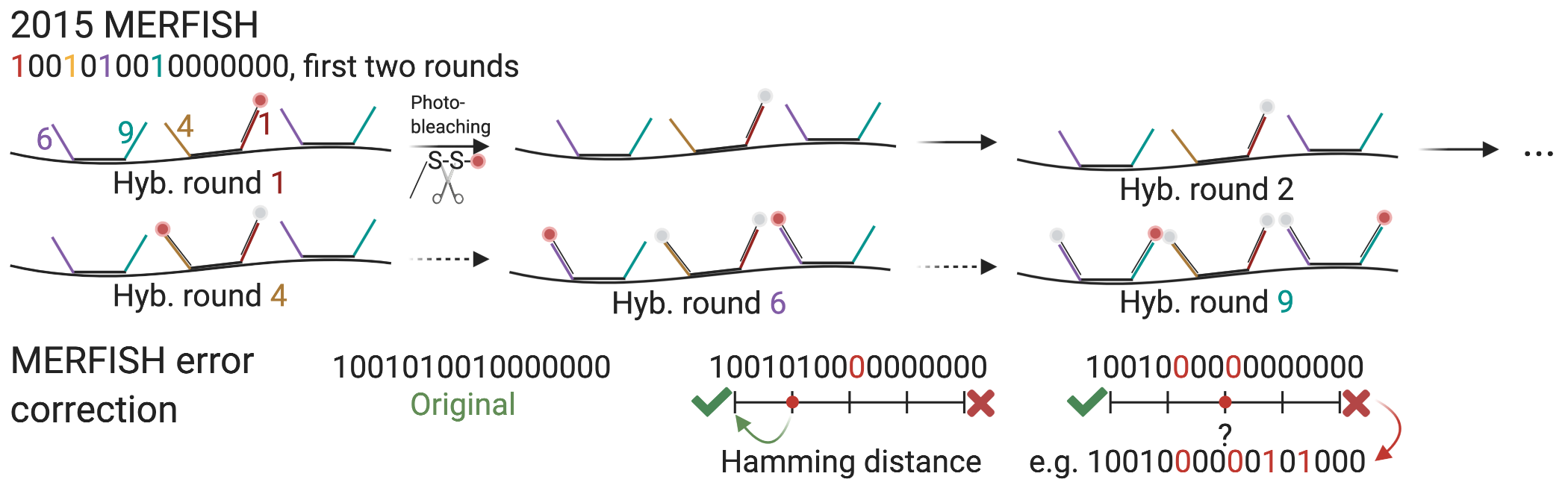
Figure 5.14: Schematic of MERFISH (K. H. Chen et al. 2015; Jeffrey R. Moffitt et al. 2016) and MERFISH error correction.

An alternative to seqFISH was developed with error correction in mind – multiplexed error-robust FISH (MERFISH) (K. H. Chen et al. 2015). In MERFISH each encoding probe has a 30 nt long region that targets the transcript, and 2 or 3 20 nt (Jeffrey R. Moffitt et al. 2016) readout sequences to bind to readout probes (Figure 5.14). First, the encoding probes are hybridized to the transcripts. For each round of hybridization, readout probes, singly labeled, are hybridized to the readout sequences on the encoding probes and imaged. Then the fluorescence of the previous round is either photobleached (version 1) (K. H. Chen et al. 2015) or when the fluorophore is bound to the readout probe with a disulfide bond, cleaved off with a reducing agent such as Tris(2-carboxyethyl)phosphine (TCEP) (version 2) (Jeffrey R. Moffitt et al. 2016). The readout probes are not stripped, and in the next round, new readout probes are hybridized to new readout sequences and imaged.

The MERFISH barcodes are binary, with “1” for a round with fluorescence, and “0” without, and must differ from other barcodes at at least 4 places, i.e. with Hamming distance of at least 4 (HD4). As missing signal is the most common error, each barcode has 4 1’s, or Hamming weight 4. This way, when one round is missing, the gene can still be uniquely identified, but when 2 rounds are missing, the remaining barcode is equally distant to 2 genes, so the error cannot be corrected (Figure 5.14). Sixteen rounds of imaging, or 16 bits, would result in 140 barcodes. In this case, there are 16 different readout sequences, and each gene is assigned 4 of them, for the 4 1’s in the barcode. If the code is expanded to 69 bits, then about 10,000 genes can be encoded, and by using 3 colors to image 3 bits per round, only 23 rounds of imaging are needed to cover the 69 bits, cutting imaging time to a third (Xia, Fan, et al. 2019). An HD2 code, i.e. barcodes are at least hamming distance 2 away from each other, can also be used, but errors can only be recognized but not corrected. All variants of MERFISH use this type of binary barcoding.

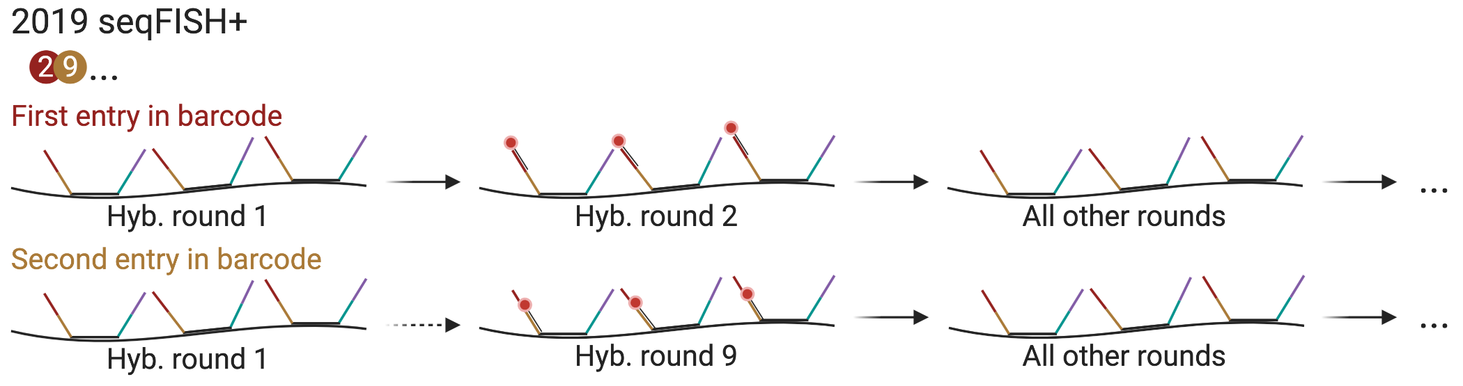
Figure 5.15: Schematic of seqFISH with pseudocolors.

More recently, a new variant of seqFISH was devised to scale up to 10,000 genes (Shah et al. 2018). The barcoding and hybridization scheme enabling such scale was first introduced in vitro in 2017 as RNA SPOTs (Chee-Huat Linus Eng et al. 2017), and was then adapted to cultured cells in 2018, targeting introns of nascent transcripts of over 10,000 genes (Shah et al. 2018). In 2019, this scheme was used to profile mature transcripts of 10,000 genes in both cell culture and the mouse brain, and with super-resolution (Chee Huat Linus Eng et al. 2019). Super-resolution beyond the diffraction limit can be achieved by computationally super-resolving the transcript spots with a radial center algorithm (Parthasarathy 2012) when spot density is very high to help with decoding barcodes; the super-resolution version is known as seqFISH+. While this new version of seqFISH can reduce optical crowding and greatly expand the palette, the super-resolution algorithm that can further reduce crowding does not have to be used to locate the transcript spots when density is low. This version of seqFISH was again used to visualize genomic loci (super-resolution) (Takei et al. 2020) and mature transcripts of a smaller number of genes (not super-resolution) (Lohoff et al. 2021).

This method is quite different from previous seqFISH variants, and is in some ways reminiscent of MERFISH. Like previous versions of seqFISH, each barcode is a series of colors, but a large number of “pseudocolors”, specifically 20 per channel in the seqFISH+ study, are used rather than the 5 fluorophores, so 3 rounds of hybridization can encode \(20^3\) or 8000 genes per channel. Any number of pseudocolors and rounds can be used depending on the number of genes profiled. Each primary probe has a 28 nt region targeting the transcript and 4 readout sites of 15 nt. Each readout site has as many different sequences as there are pseudocolors, and the 4 sites correspond to the series of 4 pseudocolors in the barcode. First, 24 primary probes are hybridized to the transcripts. Then for each place of the barcode, 20 (or whatever number of pseudocolors) rounds of hybridization with readout probes are performed, stripping with formamide between rounds. In these 20 rounds, each gene should light up only once, and its place in the 20 rounds is its pseudocolor (Figure 5.15). This way, in each image, only 1 out of 20 molecules of interest imaged in the channel fluoresce, reducing optical crowding. For the entire barcode of length 4, there would be 80 rounds of hybridization. In contrast, in MERFISH, with the 16 bit barcode, this would be 1 out of 4. Like in MERFISH, a larger number of real colors, or channels, can be used to increase throughput, to image multiple pseudocolors simultaneously. So with 3 channels, 24,000 genes can be encoded. The same error correction method as in HCR seqFISH was used, so while a barcode of length 3 is sufficient, length 4 was used.

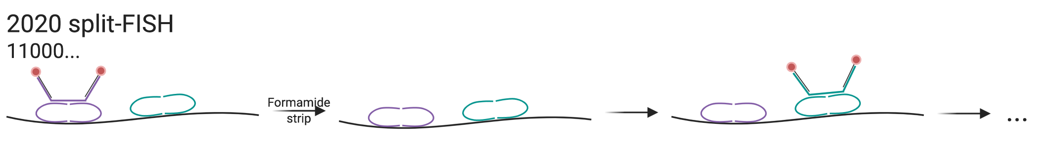
Figure 5.16: Schematic of split-FISH.

Another new method, called split-FISH (Goh et al. 2020) was devised to reduce off target hybridization, and thus background noise and some barcoding errors. For each encoding probe or bridge probe like in MERFISH, a pair of split probes hybridize to the transcript itself, inspired by the Z probes of RNAscope (Figure 5.16). Half of the split probes would bind to the transcript, and the other half bind to the bridge probe. Then as in MERFISH, the bridge probe has 2 readout sequences and singly labeled readout probes bind to the bridge probe for imaging. This method reduces off target hybridization because the bridge probe can only indirectly bind to the transcript if both of the split probes hybridize to the transcript. To encode 317 genes, 2 places out of 26 in binary barcodes are chosen to be “1”, resulting into 325 possible barcodes; 8 of them are left blank to control for false positives. Error correction is not mentioned.

Despite the availability of the above barcoding schemes, when the number of genes stained for is not too large, each gene can still be encoded by only one round of hybridization and one color. When the number of genes is larger than the number of colors, each round of hybridization stains for as many genes as there as colors, and the probes are stripped so the next round stains for a different set of genes. This has been done in osmFISH (Codeluppi et al. 2018) staining for 33 genes, in a non-barcoded adaptation of HCR-seqFISH called Spatial Genomic Analysis (SGA) (Lignell et al. 2017) staining for 35 genes, and in Expansion-Assisted Iterative Fluorescence In Situ Hybridization (EASI-FISH) 26 genes (Y. Wang et al. 2021).

5.2.2 Signal amplification

As already mentioned, in smFISH, a large number of singly labeled probes can be used to boost signal, but not all transcripts are long enough to accommodate this number of probes. Furthermore, isoform specific exons are often not long enough to accommodate these probes for isoform specific staining. Without increasing the number of probes, background reduction such as by tissue clearing, split probes (e.g. in split-FISH), and using fluorophores with colors very different from the color of autofluorescence (Jeffrey R. Moffitt et al. 2016) can increase signal to noise ratio. There are also ways to boost signals without increasing the number of probes, the most common of which are branched DNA (bDNA), rolling circle amplification (RCA), and HCR. All of these methods non-covalently attach numerous fluorophores to the probe to amplify signal. Background reduction and signal amplification can be used in conjunction.

5.2.2.1 Branched DNA

Dating back at least as far back as to 1993 (Urdea 1993), early use of bDNA in ISH was to detect low copy number of viral genomes, eventually down to single copies (Player et al. 2001). bDNA signal amplification involves several steps of hybridization (Figure 5.17). First, usually some sort of bridge probe binds to the transcript itself. Then the primary amplifier binds to the bridge probe, leaving a long overhang. Then multiple secondary amplifiers bind to the primary amplifier on the overhang of the primary amplifier, and each secondary amplifier also leaves an overhang. Finally, multiple labeled readout probes bind to each secondary amplifier. This way, space available for hybridization of the readout probes is drastically expanded, allowing for more fluorophores per unit transcript length.

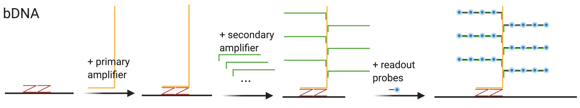
Figure 5.17: Schematic of bDNA. The Z probes are specific to RNAscope, but the other parts are generic to bDNA.

For FISH, a particularly influential bDNA method is RNAscope, introduced in 2012 for FFPE tissues, and is now commercially available from ACD (F. Wang et al. 2012). In addition to bDNA amplification, RNAscope reduces background noise from non-specific hybridization by using 2 bridge Z probes in between the transcript and the primary amplifier, so the primary amplifier will only bind when both Z probes are present. An smFISH RNAscope method has been used to profile around 1000 genes in cell culture (Battich, Stoeger, and Pelkmans 2013) and 49 genes in the mouse somatosensory cortex (Bayraktar et al. 2020), although these experiments were not highly multiplexed and only one or a handful of genes distinguishable by fluorophore color were stained for in the same cells or sections; numerous cells and sections were stained to cover all genes in the gene panels. ACD RNAscope HiPlex v2 can profile 12 targets, but without barcoding. Up to 4 targets are imaged with 4 different fluorescent channels per round of imaging, then the fluorophores are cleaved for the next round of imaging. With fresh frozen tissue, this can be applied to up to 48 targets. bDNA has also made its way into more highly multiplexed smFISH, as a variant of MERFISH (Xia, Babcock, et al. 2019). Here, the primary amplifier binds to the readout regions of the MERFISH encoding probe. Like in regular MERFISH (v2), the fluorophores are attached to the readout probes by a disulfide bond and removed by TCEP after each round of hybridization; the bDNA moiety is not removed. With bDNA amplification, only 16 probes per gene can detect about as many transcripts as with 92 unamplified probes (Xia, Babcock, et al. 2019).

5.2.2.2 Rolling circle amplification

Chronologically, the next of the popular signal amplification method is padlock probe RCA. Padlock probe was introduced in 1994 by Mats Nilsson as a way to reduce background in ISH and to detect single nucleotide variants (SNVs) (Nilsson et al. 1994). Both ends of of the padlock probe must hybridize to the target without terminal mismatches for the ligase to connect the ends of the probe to form a circle (Figure 5.18); thus padlock probe and RCA can detect SNPs and point mutations (Larsson et al. 2010; Lizardi et al. 1998). The circle encloses the target like a padlock on a string, hence the name “padlock probe”. Then probes that are not circularized are digested by an exonuclease. RCA was introduced in 1995 as a way to create tandem repeats and potentially point to origins of tandem repeats in genomes, not seeming to have signal amplification in mind (Fire and Xu 1995). A primer anneals to circularized DNA and is then elongated by \(\Phi29\) DNA polymerase, and as the polymerase goes around the circle many times, many copies of the complimentary sequences of the circle are made (Figure 5.18). In 1998, padlock probes and RCA were united to create a method of signal amplification (Baner et al. 1998; Lizardi et al. 1998).

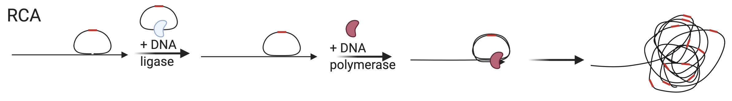
Figure 5.18: Schematic of RCA, here shown with target priming though a separate primer can also be used. Red segment is the gene barcode.

In spatial transcriptomics, padlock probe and RCA were initially used for in situ sequencing (ISS) (Ke et al. 2013), but more recently adapted to smFISH. The padlock probe with the gene barcode is hybridized to in situ reverse transcribed cDNA as in ISS and hybridization-based ISS (HybISS) (Gyllborg et al. 2020), or the mRNA itself as in SCRINSHOT (Sountoulidis et al. 2020), hybridization-based RNA ISS (HybRISS) (H. Lee et al. 2020), and barcoded oligonucleotides ligated on RNA amplified for multiplexed and parallel in situ analyses (BOLORAMIS) (S. Liu et al. 2021). RCA can be initiated with the target cDNA itself as a primer or with a separate primer when the target is mRNA. Then readout probes are hybridized to the RCA amplified gene barcode, with (Gyllborg et al. 2020) or without (Sountoulidis et al. 2020) a bridge probe. In Hyb(R)ISS and SCRINSHOT, multiple rounds of readout hybridization encode each gene with a sequence of colors as in seqFISH; although error correction is not discussed, the seqFISH error correction scheme can be easily adapted. Perhaps because of larger number of copies of the gene barcode sequence produced by RCA, Hyb(R)ISS and SCRINSHOT use 5 probes per gene, each with a 30 nt (HybISS, target sequences are proprietary information of CARTANA for HybRISS) or 40 nt (SCRINSHOT) region to target the transcript. While we are unaware of isoform specific studies conducted with Hyb(R)ISS or SCRINSHOT, isoform specific exons may more realistically accommodate the 5 probes.

5.2.2.3 Hybridization chain reaction

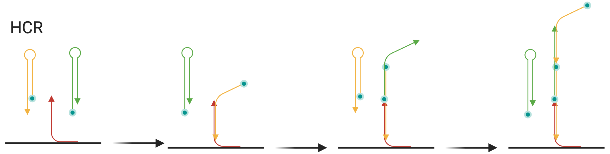
Figure 5.19: Schematic of HCR, showing 3 cycles, but this can continue indefinitely until H1 and H2 are exhausted. Arrow shows 5’ to 3’ direction.

A third signal amplification method is HCR, introduced in 2004 (Dirks and Pierce 2004), which has been adapted to seqFISH, giving rise to HCR-seqFISH. EASI-FISH also uses HCR for signal amplification. In singly labeled hairpins, the long stem is protected by the short stem, but can also hybridize with short stems of other hairpins (Figure 5.19). The long stem of H1 can hybridize to the short stem of H2, and vice versa (Figure 5.19). First, an initiator probe is hybridized to the transcript (24 per gene in the 2016 HCR-seqFISH study). Then the long stem of H1 hybridizes to the part of initiator not hybridized to the transcript, now leaving the short stem vacant. Then the long stem of H2 hybridizes to the vacant short stem of H1, and now the short stem of H2 is vacant for another H1. This cycle can continue indefinitely until H1 and H2 are depleted. This way, many fluorophores are tethered to the target transcript without increasing the number of probes bound to the transcript, thus amplifying signal.

Similarly, RCA can continue indefinitely until DNA polymerase is inhibited or removed or when deoxynucleotides are depleted. In contrast, the bDNA moiety has a controlled size and does not grow indefinitely until stopped. In both bDNA and HCR, the amplified moiety is still anchored on the target transcript. In contrast, since when the padlock probe encloses the target, the DNA polymerase is inhibited (Baner et al. 1998), the padlock must be dissociated from the target before RCA, or in the case of target priming, the target cDNA itself grows into the RCA hairball. As the hairball is not anchored to the original target, it can drift away and obscure the original location of the target. BOLORAMIS crosslinks the RCA amplicon to the cellular matrix to prevent the amplicon from drifting away.

5.2.2.4 Primer exchange reaction

Chronologically, a fourth signal amplification method is the primer-exchange reaction (PER), introduced in 2017 (Kishi et al. 2018). In PER, a hairpin with an overhang of domain A’ and double strand enclosed domain B is used. Primer A complementary to domain A’ of the hairpin anneals to the overhang, and a strand displacing polymerase copies domain B, extending domain A, thus creating a concatenation of A and B. Then the copied domain B competes with domain B in the hairpin until the concatemer AB is displaced by the hairpin’s domain B. Then another hairpin with domain B’ as the overhang can continue to extend the concatemer in the next cycle of the PER reaction. PER is used in smFISH method signal amplification by exchange reaction (SABER) (Kishi et al. 2019) for signal amplification, where the primer is the target sequence binding to the transcript has a domain A at the 3’ end, and the hairpin has a domain A’ overhang and another A and A’ in double strand instead of B and B’, so multiple copies of domain A is concatenated to the primer. Then fluorescent readout probes anneal to the multiple copies of domain A from PER, thus greatly increasing the number of fluorophores that can bind to the same transcript target. Branched probes as in bDNA can be applied to the PER concatemers for additional signal amplification. The short readout probes can be stripped without stripping the longer primary probes binding to the transcripts for multiple rounds of hybridization to image more genes than fluorophores.

5.2.3 Optical crowding

As we have seen, smFISH based spatial transcriptomics has been scaled to around 10,000 genes and can potentially be scaled to the whole transcriptome. With increasing number of mRNA molecules visualized, it’s also increasingly likely for different target molecules to be so close to each other that their fluorescent spots overlap or are even within the diffraction limit of the optical microscope and appear as one point. This is the problem of optical crowding, and some existing ways to mitigate this problem are summarized below.

As already mentioned, SRM is not susceptible to this problem (Lubeck and Cai 2012), though access to SRM is not as common as access to regular confocal or epifluorescent microscopes. Another simple strategy is to select the most highly expressed genes from RNA-seq. These genes are imaged separately with smFISH, with one color and one round of hybridization per gene instead of combinatorial barcoding, as was done in the first MERFISH study (K. H. Chen et al. 2015). However, with increasing number of highly expressed genes, this method becomes increasingly laborious. Also as already mentioned, in seqFISH+, only 1 in 60 mRNA molecules of interest light up in each channel and round of hybridization (20 pseudocolors per channel and 3 channels), and the transcript spots can be computationally super-resolved, thus reducing optical crowding (Chee Huat Linus Eng et al. 2019).

Another strategy is to allow transcript spots to overlap but computationally resolve them, as in corrFISH (Coskun and Cai 2016), BarDensr (S. Chen et al. 2021), ISTDECO (Axel Andersson et al. 2021), and Composite In Situ Imaging (CISI) (Cleary et al. 2021). In corrFISH, Transcripts of highly expressed genes encoding ribosomal proteins were visualized with sequential hybridization and 2 colors but not every gene lights up in each round of hybridization; each gene is encoded by one color and a sequence of 0’s (absence of fluorescence) and 1’s (presence) of that color. Then images from different rounds of hybridization in the same FOV are correlated to identify transcripts that are 1’s in both rounds amidst transcripts that are not 1’s in both rounds. To the best of our knowledge, after its conception, corrFISH has not been applied to generate any new high throughput dataset.

A more recent method, BarDensr, models the observed brightness of potentially mixed spots in terms of the point spread function (PSF), codebook, unknown spot density, probe washing, background, and per round per channel gain. Then the unknown spot density and deconvolution of barcodes at mixed spots are inferred by maximizing sparsity of the spots in space (most voxels don’t have spots) while keeping reconstruction loss of the observed brightness sufficiently low. BarDensr is very recently published, and, as of writing, we are unaware of studies that used the method. ISTDECO is similar but only uses a Gaussian PSF, codebook, and background.

CISI uses seqFISH-like barcoding, but does not even require spot detection. Gene abundance is computationally inferred with compressed sensing. First, an autoencoder is trained on composite images with different channels. Then in the latent space inferred by the autoencoder, the channels are decompressed with compressed sensing principles and decoded into genes with the decoder branch of the trained autoencoder. The barcodes and genes must be carefully chosen from an existing dataset. The genes must be described by a small number of coexpression modules so module activity is sparse. Inferring the sparse module activity before inferring individual gene levels at the decompression step is more tractable than directly inferring individual gene abundances.

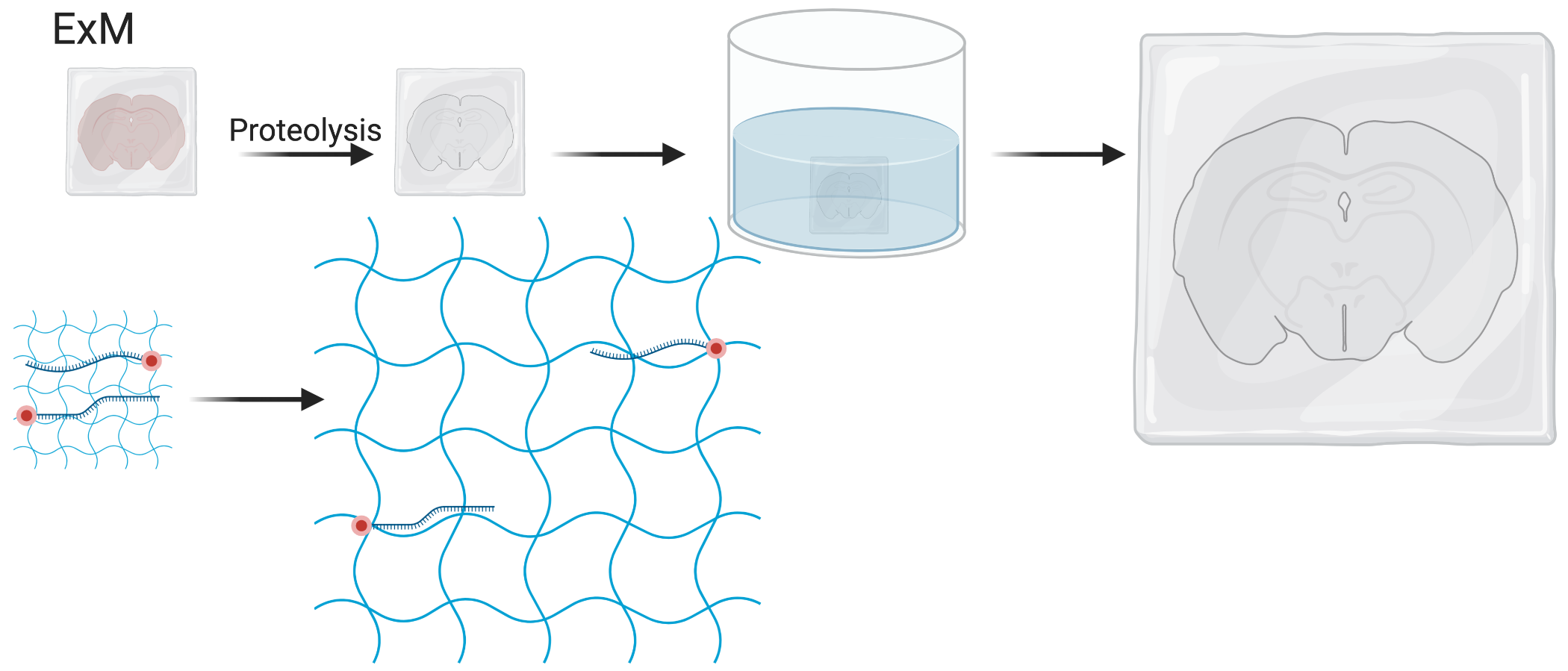
Figure 5.20: Schematic of expansion microscopy.

A strategy that has been reused is expansion microscopy (ExM). When a polyelectrolyte gel is dialyzed in water, it expands as its polymer network changes into extended conformations (F. Chen, Tillberg, and Boyden 2015). First, the tissue is infused with monomers of the gel. Then with small molecule linkers, molecules of interest such as fluorophores and RNAs can be covalently incorporated to the polymer network over the course of free radical polymerization. After the gel forms, proteins in the tissue are digested to homogenize mechanical properties of the gel and to clear the tissue to reduce autofluorescent background. Then the gel is soaked in water to expand, linearly expanding 3 to 4.5 times on each side (F. Chen, Tillberg, and Boyden 2015; F. Chen et al. 2016) (Figure 5.20). This way, transcripts attached to the gel are physically separated, avoiding optical crowding. ExM has thus been adapted to MERFISH for this purpose (G. Wang, Moffitt, and Zhuang 2018), as well as EASI-FISH. In addition, EASI-FISH was used to quantify transcripts in 300 \(\mu\)m thick brain slices and imaging was accelerated with light sheet microscopy. However, a disadvantage of ExM is that each FOV now covers less of the original tissue, thus increasing imaging time. Furthermore, the expanded gel would continue to expand during the rounds of hybridization. As the expansion is non-linear and non-isotropic, barcode decoding is challenging as it’s difficult to match transcript spots across rounds of hybridizations.

5.2.4 Usage of smFISH based techniques

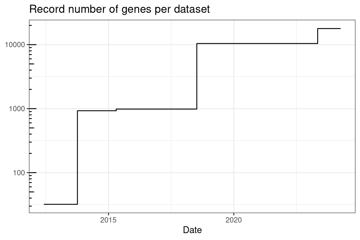
Figure 5.21: Record number of genes per dataset quantified by smFISH based techniques over time.

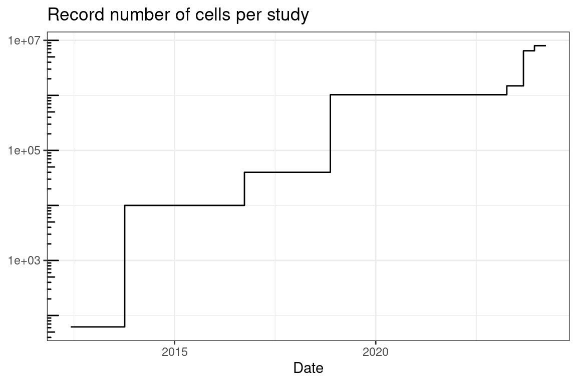
Figure 5.22: Record total number of cells per study profiled by smFISH based techniques over time.

As already noted, the number of genes whose transcripts can be possibly quantified simultaneously in the same piece of tissue with highly multiplexed smFISH based technology has increased over time (Figure 5.21). The number of cells that can be imaged in one study has also increased (Figure 5.22). However, in practice, the actual number of genes and cells profiled has not significantly increased (Figure 5.23, Figure 5.24). These plots only show papers that reported the number of cells and genes in the main text; if we download and process all publicly available datasets associated with such papers, the trends might change, although figures of papers that do not report the number of cells (number of genes is usually reported in smFISH and ISS studies) don’t seem to indicate that the trend would change significantly. Moreover, as discussed in Section 5.8, some of the studies used smFISH based methods to visualize DNA loci and 3D chromatin structure alongside transcripts. The number of genes here is for the transcripts, including when only introns are targeted.

An earlier version of the plot of number of genes over time plotted the mean number of genes for each study, due to difficulty in defining what constitutes a dataset. However, since that version caused confusion as sometimes one study profiled very different number of genes in different experiments, we decided to give some definition of “dataset” and not to plot the mean. Here a “dataset” means either a different tissue, cell type, experimental or clinical condition, or a separate experiment profiling a different number or set of genes in the same study. One dataset can involve multiple sections and individuals.

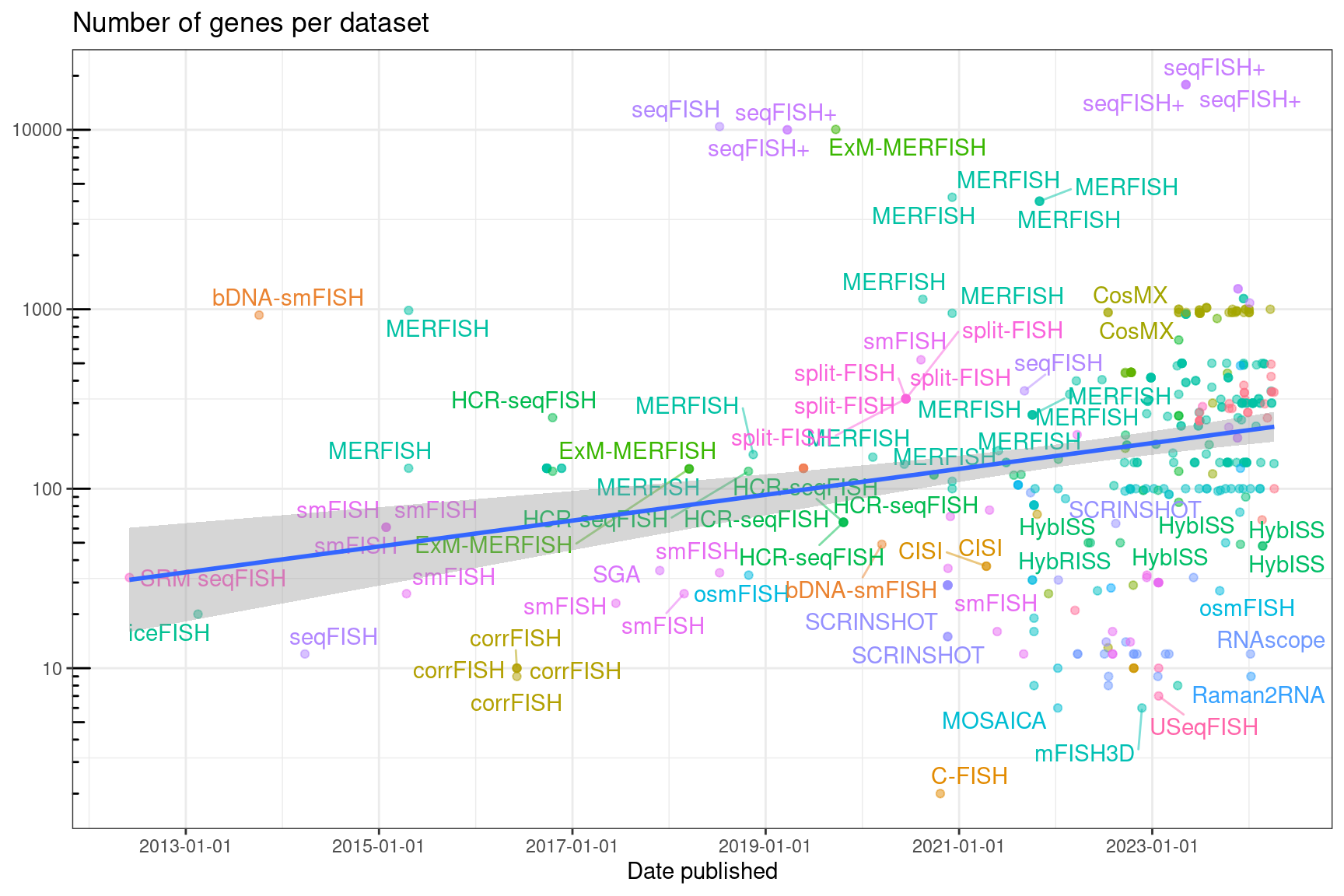
Number of genes per datasets in each study, over time. Gray ribbon is 95% confidence interval (CI). The points are translucent; more opaque points are multiple datasets from the same study.

Figure 5.23: Number of genes per datasets in each study, over time. Gray ribbon is 95% confidence interval (CI). The points are translucent; more opaque points are multiple datasets from the same study.

The trend line looks pretty flat. Although studies quantifying a very large number of genes tend to be recent, many other studies profiling fewer genes pulled the line down. As of August 2023, the slope has finally become significantly different from 0, showing a very slow trend of increasing number of genes per dataset but most datasets profile a few hundred genes. For a long time, the slope (with all data, outliers and all) had not been significantly different from 0 (t-test), after log transforming the number of genes per dataset.

## 
## Call:
## lm(formula = log(n_genes) ~ date_published, data = smfish)
## 
## Residuals:
##     Min      1Q  Median      3Q     Max 
## -4.1344 -0.6873  0.2039  0.8417  4.8027 
## 
## Coefficients:
##                  Estimate Std. Error t value Pr(>|t|)    
## (Intercept)    -3.599e+00  1.752e+00  -2.054   0.0406 *  
## date_published  4.541e-04  9.157e-05   4.959 1.06e-06 ***
## ---
## Signif. codes:  0 '***' 0.001 '**' 0.01 '*' 0.05 '.' 0.1 ' ' 1
## 
## Residual standard error: 1.451 on 387 degrees of freedom
##   (33 observations deleted due to missingness)
## Multiple R-squared:  0.05974,    Adjusted R-squared:  0.05731 
## F-statistic: 24.59 on 1 and 387 DF,  p-value: 1.063e-06

How total number of cells profiled in each study that reported the number of cells in the main text is shown here. The total number across datasets is used because sometimes number of cells per dataset is not reported.

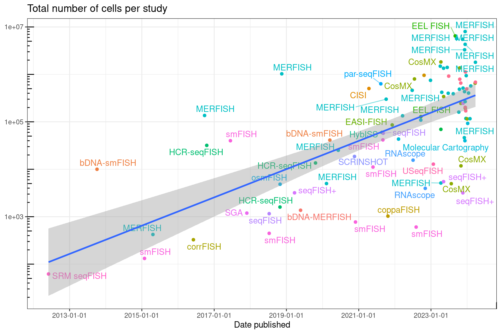
Figure 5.24: Total number of cells per study profiled by smFISH based techniques over time.

After log transforming the total number of cells per study (when reported), whose distribution is very right skewed, it does seem that the total number of cells increased with time (Figure 5.24). New smFISH based techniques in our database since 2021 are all optimized for features other than larger number of genes and are applied to relative small numbers of genes in demonstration. For instance, EASI-FISH is optimized for thick brain sections (Y. Wang et al. 2021). par-seqFISH is optimized for bacteria (Dar et al. 2021). CISI is optimized for reducing the number of imaging cycles and avoiding direct spot calling and has not been demonstrated on large number of genes (Cleary et al. 2021). The distinctive feature of MOSAICA is to use both the color and the lifetime of the fluorophores and is only demonstrated to be 10-plex (Vu et al. 2021). Recent applications of existing techniques also tend to feature larger number of cells but only hundreds of genes (e.g. 368 genes in (Choi et al. 2022)), where the MERFISH dataset is complementary to scRNA-seq datasets of the same tissue, using marker genes from scRNA-seq clusters.

## 
## Call:
## lm(formula = log(n_cells) ~ date_published, data = sum_cells)
## 
## Residuals:
##     Min      1Q  Median      3Q     Max 
## -5.2714 -1.2602 -0.0281  1.4722  4.7155 
## 
## Coefficients:
##                  Estimate Std. Error t value Pr(>|t|)    
## (Intercept)    -2.438e+01  4.306e+00  -5.661 1.81e-07 ***
## date_published  1.877e-03  2.263e-04   8.294 1.08e-12 ***
## ---
## Signif. codes:  0 '***' 0.001 '**' 0.01 '*' 0.05 '.' 0.1 ' ' 1
## 
## Residual standard error: 2.067 on 89 degrees of freedom
## Multiple R-squared:  0.436,  Adjusted R-squared:  0.4296 
## F-statistic: 68.79 on 1 and 89 DF,  p-value: 1.08e-12

MERFISH is the smFISH based technique used in the most institutions (Figure 4.7), although most of the smFISH based techniques barely spread beyond their institutions of origin, if at all (Figure 5.26). The following advantages and disadvantages of smFISH based techniques may explain these trends in usage. Advantages and disadvantages of individual smFISH based techniques reviewed so far are summarized in Table 5.1.

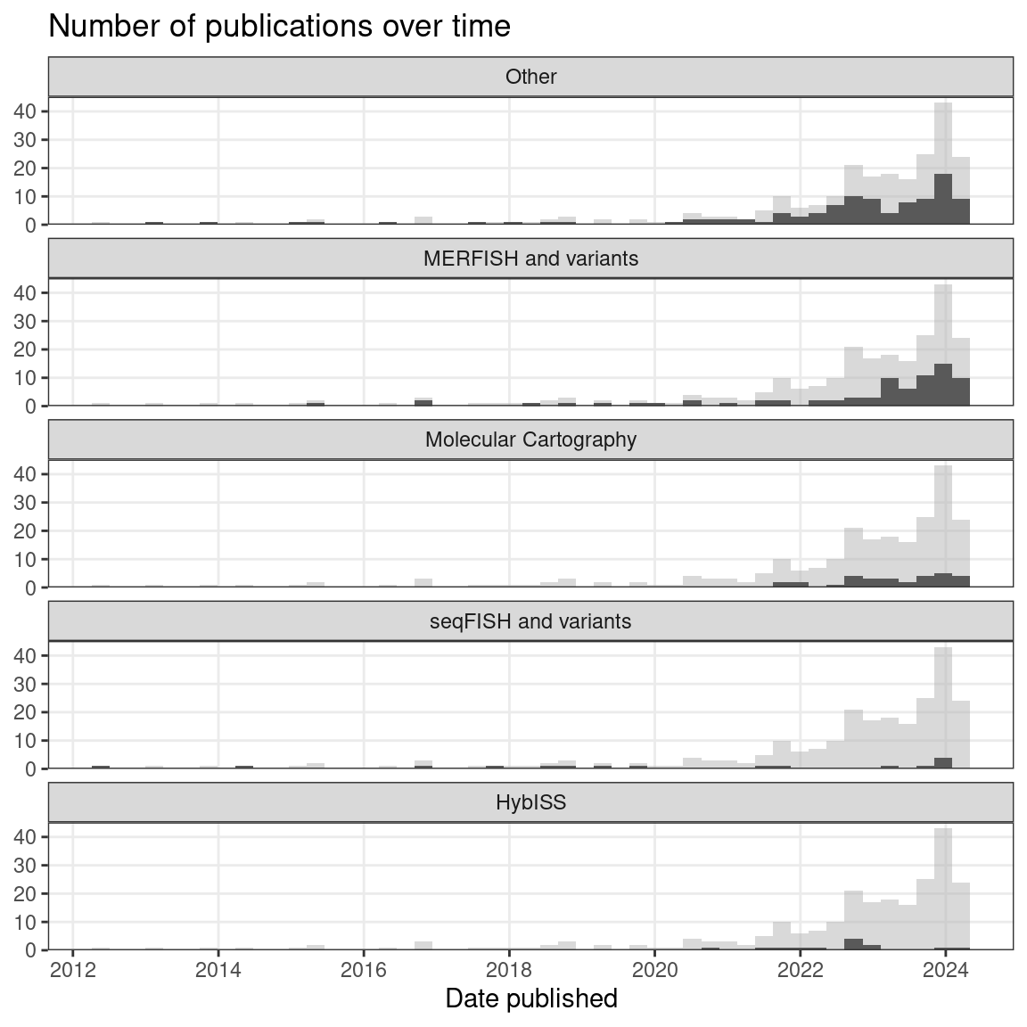
Number of publications over time, broken down by technique type. Preprints are included, and the gray histogram in the background is the overall trend of all smFISH based techniques. Bin width is 90 days.

Figure 5.25: Number of publications over time, broken down by technique type. Preprints are included, and the gray histogram in the background is the overall trend of all smFISH based techniques. Bin width is 90 days.

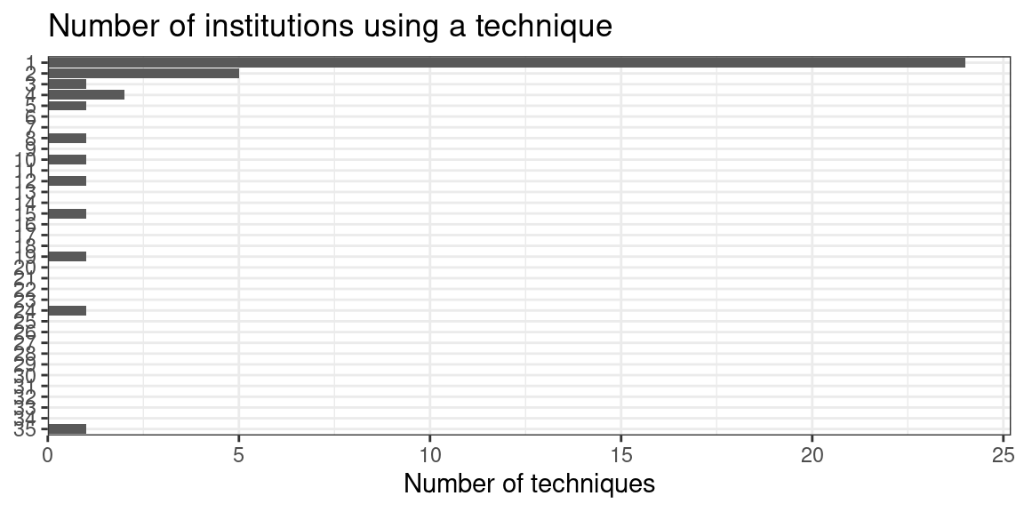
Number of techniques that have been used by each number of institutions; most techniques have only been used by 1 institution, i.e. the institution of origin.

Figure 5.26: Number of techniques that have been used by each number of institutions; most techniques have only been used by 1 institution, i.e. the institution of origin.

MERFISH has been commercialized by Vizgen and has spread much more far and wide than seqFISH and HybISS; another commercial technology, Molecular Cartography also also spread far and wide (Figure 5.27). While MERFISH is mostly used in the US, Molecular Cartography is mostly used in Europe, in accordance with the location of their companies.

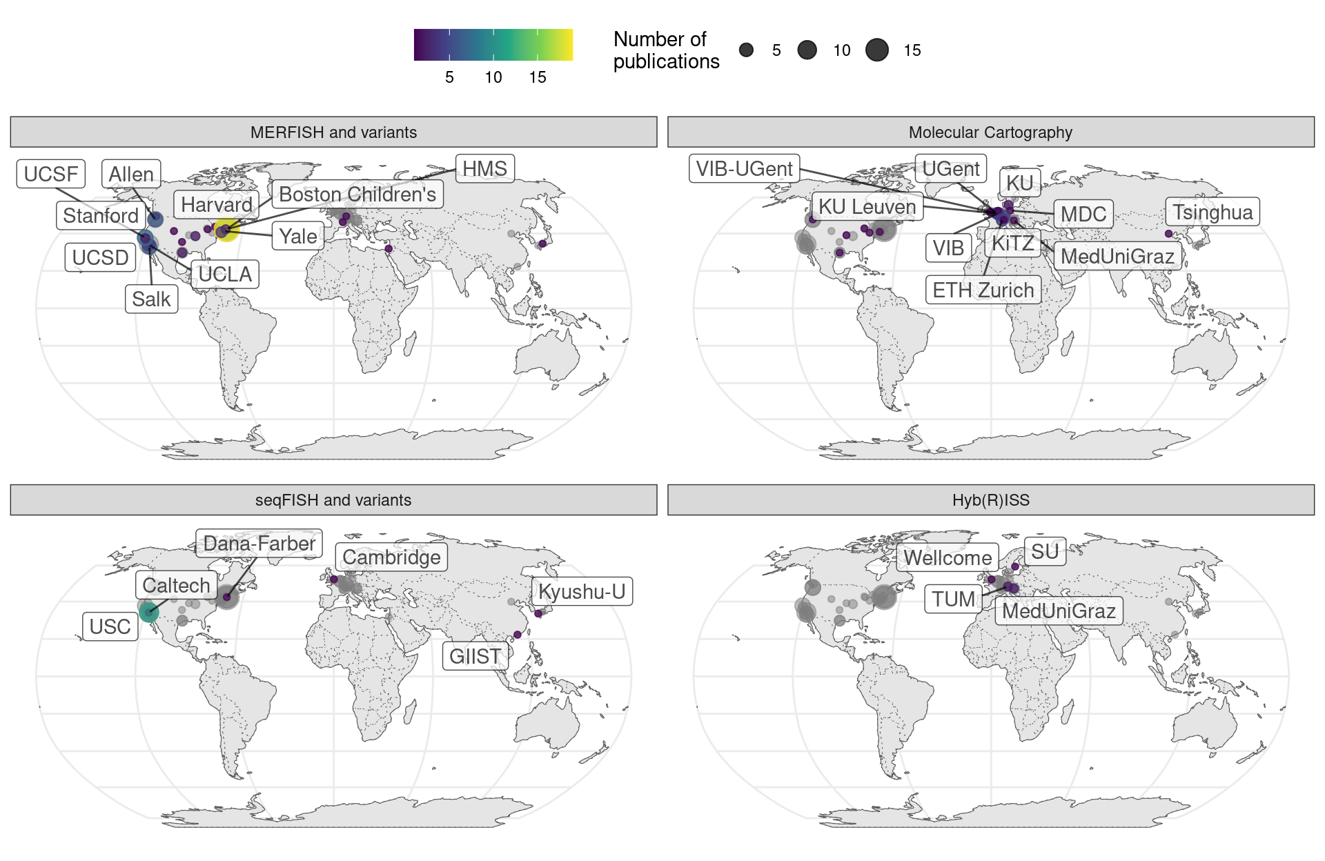
Geographical locations of institutions that used certain techniques. Point area is proportional to number of publication from the city of interest. Gray points in the background is all publications using smFISH based techniques. The cities and institutions labeled are those of the first author. Note that for seqFISH, the hidden Markov random field (HMRF) study at Dana Faber (Q. Zhu et al. 2018) and the mouse embryo study (Lohoff et al. 2021) had collaboration with Long Cai’s group at Caltech, so the dataset was most likely still collected at Caltech.

Figure 5.27: Geographical locations of institutions that used certain techniques. Point area is proportional to number of publication from the city of interest. Gray points in the background is all publications using smFISH based techniques. The cities and institutions labeled are those of the first author. Note that for seqFISH, the hidden Markov random field (HMRF) study at Dana Faber (Q. Zhu et al. 2018) and the mouse embryo study (Lohoff et al. 2021) had collaboration with Long Cai’s group at Caltech, so the dataset was most likely still collected at Caltech.

SmFISH based techniques have the following advantages. First, smFISH, especially with larger number of probes, have nearly 100% detection efficiency of transcripts (Lubeck and Cai 2012), i.e. detecting almost all transcripts that are present. Different ways to evaluate efficiency of spatial transcriptomics techniques have been reported. The reported “efficiency” of MERFISH was estimated by the average ratio between the number of transcripts per segmented cell detected by MERFISH and those detected by smFISH in the same cell type for 10 genes. With combinatorial barcoding, however, the efficiency is decreased. Studies for other techniques may use different ways to estimate efficiency. Compared to smFISH, MERFISH version 2 with HD4 code has about 95% detection efficiency on 130 genes and 92 probes per gene, although the efficiency dropped to ~25% with the HD2 code that can encode nearly 1000 genes but can only identify but not correct errors (Jeffrey R. Moffitt et al. 2016; Foreman and Wollman 2019). When scaled to 10,050 genes, MERFISH has around 79% detection efficiency (Xia, Babcock, et al. 2019). As for HCR-seqFISH, the efficiency is around 84% (smFISH and HCR-seqFISH were performed in the same cell for 5 genes) (Shah et al. 2016), and for seqFISH+, around 49% (slope of line fitted to average transcript count per cell in seqFISH+ vs. smFISH for 60 genes) (Chee Huat Linus Eng et al. 2019). Nevertheless, this is much better than the efficiency of ST, which is around 6.9% compared to smFISH in the 2016 ST study (transcript counts for 3 genes in ST spots were compared to those from smFISH of 100 \(\mu\)m diameter discs at comparable brain regions in an adjacent section) (Ståhl et al. 2016). To put the 6.9% in context, from ERCC spike ins and in some cases comparison to smFISH, scRNA-seq methods such as Drop-seq, 10X, inDrop, CEL-seq, and CEL-seq2 have capture efficiency of between 3% and 25% (Macosko et al. 2015; Zheng et al. 2017; A. M. Klein et al. 2015; Hashimshony et al. 2016; Grün, Kester, and Oudenaarden 2014). Thus smFISH based spatial transcriptomics methods can be much more efficient than scRNA-seq, though efficiency of RCA based smFISH compared to regular smFISH has not been reported.

Second, since individual transcripts are imaged and counted, smFISH based methods are highly quantitative and records subcellular localization of transcripts. While most smFISH based spatial transcriptomics studies analyze data at the cellular gene count level, not using subcellular transcript localization, cells have been shown to show great variation in subcellular localization of transcripts of the same set of genes and a number of “archetypal” patterns have been described (Samacoits et al. 2018; Stoeger et al. 2015; Cabili et al. 2015).

The following disadvantages may explain why smFISH based spatial transcriptomics has not been widely used on large number of genes (Figure 5.23), and why MERFISH is the most used technique (Figure 5.25). First, multiple rounds of hybridization and high magnification mean that data collection is time consuming. MERFISH version 2 greatly sped up imaging, as version 1 requires higher magnification and needs to photobleach fields of view (FOV) one at a time; one FOV in version 1 is 40 \(\mu\)m \(\times\) 40 \(\mu\)m, while one FOV in version 2 is 223 \(\mu\)m \(\times\) 223 \(\mu\)m. Version 2 also cut imaging time in half by using 2 colors, targeting 2 bits per round. This way, for 130 genes and 40,000 cells, MERFISH took about 18 hours (Jeffrey R. Moffitt et al. 2016), while HCR-seqFISH would take days because of overnight hybridization after probes are stripped for each round of hybridization although the seqFISH barcode is much shorter. When scaled to 10,000 genes, MERFISH takes 23 rounds of hybridization (Xia, Fan, et al. 2019), while seqFISH+ takes 80 rounds (Chee Huat Linus Eng et al. 2019), although because ExM was used for MERFISH in this case to reduce optical crowding, expanding the area to be images ~4 folds, the actual imaging time of ExM-MERFISH and seqFISH+ here may have been comparable. Perhaps MERFISH has been scaled to larger number of cells and used in more studies beyond the institution of origin (Figure 5.27) because of the higher detection efficiency and shorter imaging time.

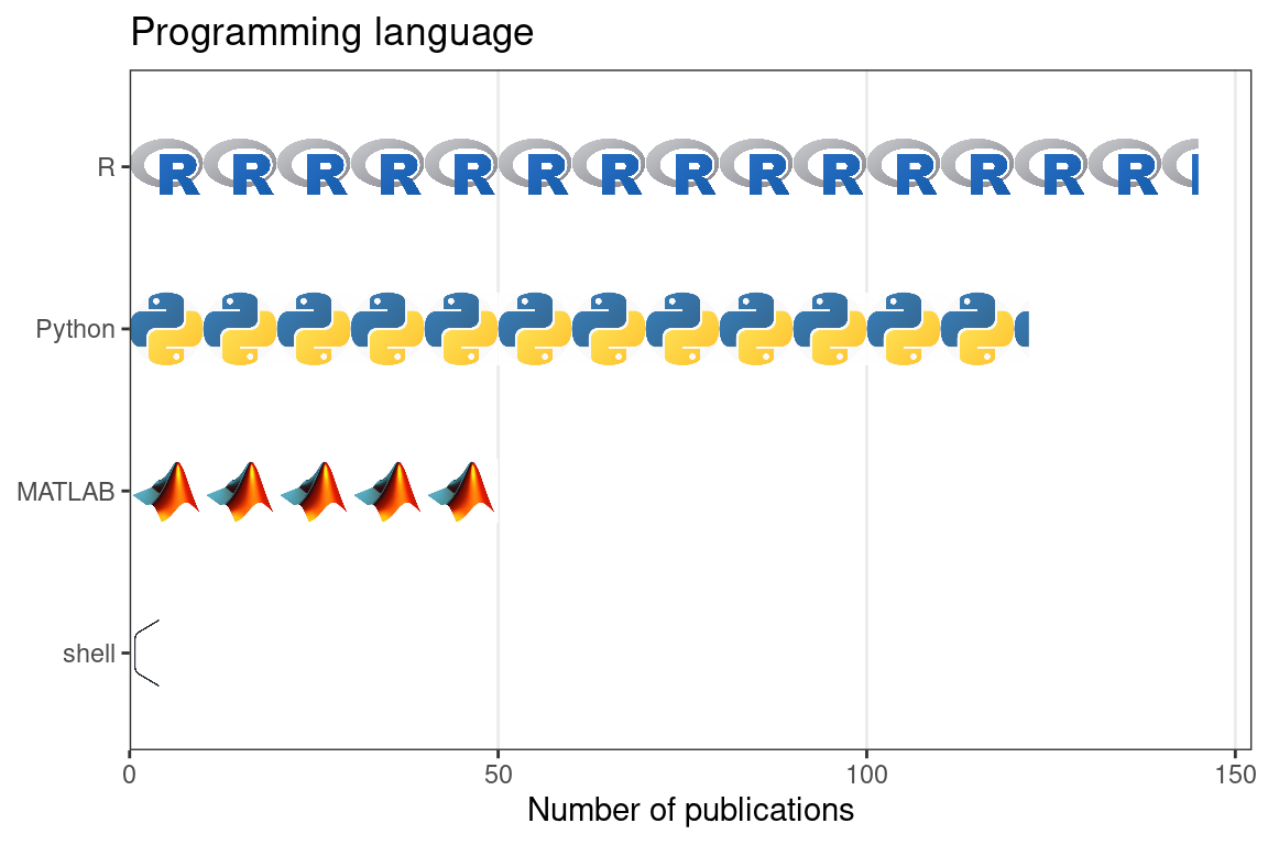
Number of publications using smFISH based techniques that used each of the 5 most common programming languages. Each icon stands for 10 publications.

Figure 5.28: Number of publications using smFISH based techniques that used each of the 5 most common programming languages. Each icon stands for 10 publications.

Second, with increasing area of tissue and number of genes covered, smFISH based spatial transcriptomics generates terabytes of images – for each FOV, there is an image for each channel, z-plane, and round of hybridization. Images from the MERFISH dataset of 40,000 cells and 130 genes took 2 to 3 days to process on a multi-core server, although the number of cores was not stated (Jeffrey R. Moffitt et al. 2016). In contrast, it takes hours, or even just minutes, to process the fastq files of a scRNA-seq dataset to get the gene count matrix (Melsted et al. 2021), nor do the fastq files take up so much disk space. So for the user, processing the most upstream form of data is much more challenging for highly multiplexed smFISH than scRNA-seq. Until 2019, software to process such images and to decode the combinatorial barcodes was typically written in the proprietary programming language MATLAB (Figure 5.28), and poorly documented, so it was difficult for people outside the lab of origin to use.

More recently, Python is replacing MATLAB as the programming language of choice to write such image processing software. The Chan Zuckerberg Initiative developed starfish in Python as a unified framework to process smFISH based spatial transcriptomics data (Perkel 2019). However, image processing pipelines specific to each technology have been developed instead, such as MERlin for MERFISH (Xia, Fan, et al. 2019) and IRIS for ISS (C. Zhou et al. 2020), and image stitching is performed separately such as with MIST (Chalfoun et al. 2017) or BigStitcher (Hörl et al. 2019) if needed as starfish does not directly support multiple FOVs. starfish has been used by the HybISS group (Bruggen et al. 2021; Gyllborg et al. 2020) for spot calling, decoding, and cell segmentation, and by the CISI group for spot calling (Cleary et al. 2021) and CellProfiler for cell segmentation. In contrast, for scRNA-seq, there are popular data processing tools that apply across technologies, such as STAR (wrapped by Cell Ranger) (Dobin et al. 2012), alevin (Srivastava et al. 2019), and kallisto (Melsted et al. 2021). Furthermore, even with an open source and interoperable image processing pipeline, cell segmentation, which is essential to obtaining the gene count matrix commonly used in data analysis, is challenging.

Third, custom fluidics systems have been used for the numerous rounds of hybridization (Chee Huat Linus Eng et al. 2019; Jeffrey R. Moffitt et al. 2016; Codeluppi et al. 2018). These custom fluidics and pump systems are not commercially available and need to be built by any lab that wishes to adopt the smFISH based technologies. To the best of our knowledge, there are no core facilities that perform smFISH based spatial transcriptomics. Thus for the user, adopting an smFISH based spatial transcriptomics technique means not only learning a new syntax to process images, made difficult in some cases by the cost of MATLAB and lack of documentation, but also setting up a complex custom fluidics system integrated to a microscope, which may not be feasible at microscopy cores. However, this is changing with commercial Vizgen MERFISH, the Rebus Esper spatial omics platform, Molecular Cartography of Resolve Biosciences, 10X Xenium, and Nanostring CosMX, with convenient automated imaging machines and reagent kits. Rebus Esper was used to automate osmFISH in (Bhaduri et al. 2021), and claims to have less than one hour of hands on time and be able to return a gene count matrix for 100,000 cells with spatial coordinates of the cells within 2 days. While Molecular Cartography is smFISH based, it’s not clear from its website how it works and it only profiles 100 genes. Aria from Fluigent can also be potentially used to automate highly multiplexed FISH. MERFISH and Molecular Cartography have spread far and wide after commercialization, and we expect other commercial smFISH platforms to spread as well.

Fourth, to profile large numbers of genes, numerous probes need to be designed, especially when dozens of probes are used for each gene to enhance signal. Probes with fluorophores are expensive as well and larger quantity of them are needed with signal amplification. These probes are an expensive one time purchase, and might not be worthwhile if a lab does not perform highly multiplexed smFISH very often. A core facility with a good collection of probes can reduce cost to individual labs, but to reiterate, as of writing, we are unaware of any core facility performing highly multiplexed smFISH techniques such as MERFISH (except NeuroTechnology Studio at Brigham Health for MERFISH) and seqFISH. Cost of probes could be a reason why recent applications of highly multiplexed smFISH techniques did not profile larger number of genes. Finally, smFISH based techniques require a pre-defined list of genes and probes, so unlike in RNA-seq, novel transcripts would be missed.

Table 5.1: Pros and cons of smFISH based techniques.
Technique	Pro	Con
HCR-seqFISH	Relatively high efficiency (84%), fewer rounds of hybridization, error correction	Lower efficiency than MERFISH, time consuming to re-hybridize probes to target after stripping
seqFISH+	Avoids optical crowding, scalable	Lower efficiency (49%), numerous rounds of hybridization
MERFISH	High efficiency (95%) with HD4 code, error correction, version 2 relatively fast, scalable, commercialized	Numerous rounds of hybridization, numerous probes requiring long transcripts though this is resolved by bDNA signal amplification
ExM-MERFISH	Avoids optical crowding, clears tissue	Each FOV contains less of the original tissue
HybISS	Only 5 probes per gene, applicable to isoform specific exons, padlock probe reduces background, lower magnification when imaging (20x and 40x, while MERFISH uses 60x), can discern SNPs	Error correction not reported, amplicon takes up space and might drift away if not cross linked
HybRISS	Avoids inefficiency of reverse transcription, better signal to noise ratio and more transcripts detected then HybISS.	Padlock probe sequences are proprietary to CARTANA
bDNA-smFISH	Commercial RNAscope kit, reduces background and amplifies signal, amplified moiety does not grow indefinitely	Except for bDNA-MERFISH, it has not been used in a highly multiplexed setting

So far we have reviewed studies that showcase new techniques and technical improvements such as signal amplification and resolving optical crowding. Some smFISH based techniques have been used in studies that focus on biological problems rather than new techniques. HCR-seqFISH has been used twice in biological studies, in chicken neural tube (35 genes) (Lignell et al. 2017) and mouse T cell precursors (65 genes) (W. Zhou et al. 2019) though both were conducted within Caltech, the institution of origin. Moreover, spatial location of cells is not necessarily a reason to use HCR-seqFISH; Zhou et al. used HCR-seqFISH because of the high detection efficiency compared to scRNA-seq in dissociated FACS sorted T cell progenitors, so when spatial information is already lost. More recently, pseudocolor seqFISH was used in a mouse embryo atlas at University of Cambridge (though Long Cai is still a coauthor), finally moving beyond the stage of testing into new biological research (Lohoff et al. 2021). Combinatorial barcoding has also been used to profile bacterial species in the microbiome by targeting rRNAs, though this does not profile the transcriptome, nor is it single molecular (Shi et al. 2020; Z. Cao et al. 2021). For spatial transcriptome in bacteria, a new version of seqFISH, par-seqFISH, was developed to profile 105 genes in the biofilm bacterium Pseudomonas aeruginosa (Dar et al. 2021). This may open the way to spatial transcriptomics in not only biofilms, but in the microbiome in general.

MERFISH has been used more broadly in biological studies. Within Harvard, the institution of origin, MERFISH has been used to create atlases of the hypothalamic preoptic region (155 genes) (Jeffrey R. Moffitt et al. 2018) and the primary motor cortex (MOp) (258 genes) (M. Zhang et al. 2020) in mice, and adapted to stain for chromatin conformation and transcription foci (introns) (Su and Song 2020). Outside Harvard (Figure 5.27), MERFISH has been used to study how gene expression variability relates to cell state in cell culture (Foreman and Wollman 2019) and used in conjunction with smFISH based chromatin tracing to study the relationships between chromatin compartmentalization and gene expression (M. Liu et al. 2020).

After its inception, HybISS became part of a single cell atlas of the developing mouse nervous system (Manno et al. 2021). This atlas is mostly scRNA-seq data, but 119 genes were stained with HybISS to validate secondary organizers discovered via scRNA-seq. As part of the HCA, HybISS has also been used for the human adult temporal lobe (Langseth et al. 2021) and fetal forebrain (Bruggen et al. 2021).

5.3 In situ sequencing

In contrast to smFISH based techniques, techniques reviewed in this section determine the sequences of the target transcript or the gene specific barcode by in situ sequencing by ligation (SBL) or sequencing by synthesis (SBS) to distinguish between transcripts of different genes. This section reviews 3 in situ SBL strategies, SOLiD, cPAL, and SEDAL, and the spatial transcriptomics techniques using them.

SBL relies on the specificity of the DNA ligase, so ligation only occurs when both sequences to ligate match the template in the vicinity of the site of ligation. Prior to SBL, this specificity was used to detect SNVs that would otherwise be missed as ISH probes can tolerate some mismatches. A technique using ligation of two oligonucleotides to detect SNVs was introduced in 1988 by Ulf Landegren (Landegren et al. 1988), laying the foundation of SBL (Figure 4.3). The padlock probe came in the same tradition of SNV detection, and Mats Nilsson worked with Landergren when creating the padlock probe (Nilsson et al. 1994).

Almost all spatial transcriptomics techniques based on SBL require in situ reverse transcription of the mRNAs as ligation with RNA as template is inefficient. As already mentioned in Section 5.1.1.2, IVT amplification of transcripts from single cells for expression profiling originated in the Eberwine group (Gelder et al. 1990; Eberwine et al. 1992), where rather than LCM, the cDNAs from the single cells were reverse transcribed in situ during electrophysiological recording before the cellular content was aspirated for IVT amplification. This was built upon the in situ reverse transcription technique from the Eberwine group in 1988 (Tecott, Barchas, and Eberwine 1988), where the cDNA of proopiomelanocortin (POMC) was radiolabeled so the spatial distribution of the mRNA was visualized on an autoradiograph. This made most in situ SBL techniques possible, which instead of radioactivity, use gene barcodes to locate the transcripts in a multiplexed and safer way.

5.3.1 SOLiD and FISSEQ

The earliest proposal of SBL we are able to locate is a patent filed in 1995 describing a method similar to sequencing by oligo ligation detection (SOLiD). An initiator oligonucleotide hybridizes to the template to be sequenced, and is extended by ligation to a 9-mer probe with a label such as a fluorophore that indicates one or two nucleotides of the probe (Macevicz 1995). The probe has a blocking moiety so only one probe is ligated in each cycle. Then the blocking moiety is removed so the initiator can be further extended by ligation in the next cycle. As mismatches in the probe inhibit ligation, the nucleotide of interest in the probe can be read off from the label after probes that are not ligated are removed. This can determine every 9th nucleotide in the template, and with 9 different initiators, each out of phase by one nucleotide, the sequence of the entire template can be determined. However, this method existed only on paper, while since 2006, Applied Biosystems (Applera) seemed to have developed SOLiD independently from that patent after acquiring Agencourt, which developed a sequencing by ligation method that would be the foundation of SOLiD (Alsup 2009).

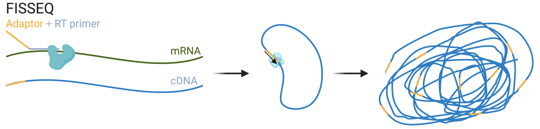
Figure 5.29: Schematic of RCA in FISSEQ.

In 2014, single cell resolution and transcriptome wide spatial transcriptomics was far out of reach (Figure 5.21). An attempt to reach this goal was fluorescent in situ sequencing (FISSEQ) (J. H. Lee et al. 2014). A universal adapter and random hexamer reverse transcription (RT) primer was hybridized to the mRNAs to reverse transcribe them into cDNA (Figure 5.29). Then the cDNA, now with the adaptor on the 5’ end, is circularized, and amplified with RCA with a primer complementary to the adaptor. Then again, with sequencing primers receding into the adaptor, SOLiD is used to sequence the cDNA amplicons in situ.

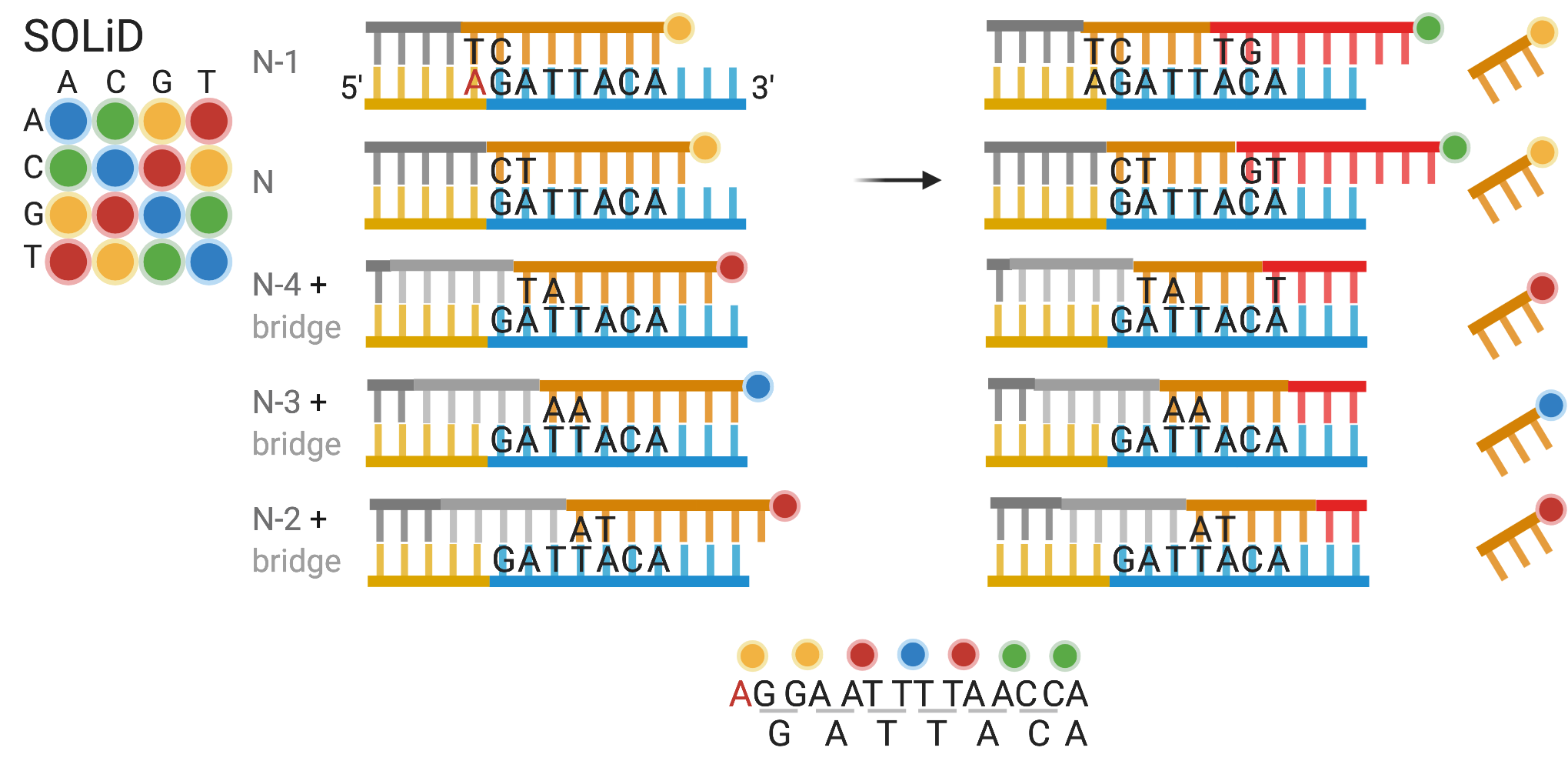
Schematic of SOLiD sequencing, determining the sequence GATTACA. The rows are arranged in the order of 5' to 3' positions of the first fluorescent probe, but the actual hybridization and ligation can take a different order. As part of the constant region, the 'A' highlighted in red is known.

Figure 5.30: Schematic of SOLiD sequencing, determining the sequence GATTACA. The rows are arranged in the order of 5’ to 3’ positions of the first fluorescent probe, but the actual hybridization and ligation can take a different order. As part of the constant region, the ‘A’ highlighted in red is known.

In SOLiD, color of the fluorophore encodes the two 3’-most bases of 8-mer probes with other bases degenerate (Figure 5.30). Once a probe perfectly matching the target right after the primer, the probe is ligated to the primer and the fluorescent signal is recorded. Then the fluorophore and the nearest 3 bases of the probe are cleaved off. In the next cycle, a new matching probe is ligated to the now extended primer. This is continued until the end of the target, for 7 cycles per primer in the case of FISSEQ (J. H. Lee et al. 2015). For the first 7 cycles, the primer matches the adaptor (N). Then the primer N, extended for 7 cycles is stripped, and a new primer receding one nucleotide to the 5’ end of the adaptor (N-1) is added in cycle 8. Again 7 cycles of ligation are performed and the extended primer N-1 is stripped after cycle 14 to make room for N-2. For N-2, N-3, and N-4, a bridge oligo is used so the target with unknown sequence, rather than the adaptor with known sequence, is interrogated by the probes. With N through N-4, the entire target is covered. With the fluorescent signals recorded from the rounds of ligation, and the knowledge of the last nucleotide of the adaptor interrogated by the first ligation to primer N-1, the sequence of the target can be determined. Figure 5.30 shows how SOLiD determines the sequence “GATTACA”. As already mentioned in the smFISH section, with increasing number of genes profiled, optical crowding is increasingly a problem. To mitigate optical crowding, the primer N can have one or more degenerate bases at the 5’ end reaching into the target; with one degenerate base, only 1/4 of the amplicons are sequenced. With two bases, this would be 1/16. This is repeated to cover all transcripts, but increases imaging time.

While FISSEQ may seem a promising approach to reach the goal of single cell resolution and transcriptome wide spatial transcriptomics that unlike smFISH based techniques, is not limited by pre-defined gene panels, it has been largely dormant since its inception due to the following disadvantages. First, SOLiD has fallen out of favor because of limited read length when used in situ (5-30 nt), propagation of errors from previous cycles (Alon et al. 2021), and difficulty in sequencing panlindromic sequences (Giani et al. 2020). SOLiD was chosen for FISSEQ because it works well at room temperature; though SBS supports longer read lengths, it requires a heated stage (J. H. Lee et al. 2015). Second, FISSEQ is extremely inefficient, over 20 times less sensitive than scRNA-seq and two orders of magnitude less sensitive than 2013 Nilsson ISS (discussed later in this section) (J. H. Lee et al. 2015), in part because of inefficiency of random RT priming (J. H. Lee et al. 2014) and tight packing of amplicons (Alon et al. 2021). Furthermore, as ribosomal RNA (rRNA) is not depleted, ~40-80% of FISSEQ reads are rRNA (J. H. Lee et al. 2014, 2015). As about 200 mRNA reads are detected per cell in FISSEQ without rRNA depletion, compared to about 40,000 in scRNA-seq, and suppose detection efficiency of scRNA-seq is 10%, then detection efficiency of FISSEQ might be around 0.005% (J. H. Lee et al. 2015). Third, highly abundant genes involved in translation and splicing is depleted in FISSEQ compared to bulk RNA-seq (J. H. Lee et al. 2014). Finally, FISSEQ imaging is time consuming, taking 2 to 3 weeks if performed manually (J. H. Lee et al. 2015).

With expansion microscopy, the idea of FISSEQ was revived in ExSeq (Alon et al. 2021). Just like in ExM-MERFISH, transcripts are incorporated into a polyelectrolyte gel, which is expanded, so the amplicons are no longer so tightly packed. This eliminated the depletion of highly abundant genes compared to bulk RNA-seq, and the detection efficiency and proportion of rRNA reads of ExSeq seem on par with randomly primed bulk RNA-seq of adjacent sections. In addition to SOLiD sequencing as in FISSEQ, the amplicons are also sequenced ex situ with Illumina SBS. The in situ sequences are matched to ex situ sequences and only unique matches are kept, to more effectively align amplicons to the genome and to localize mRNA sequence variations such as alternative splicing that are more difficult to detect with SOLiD’s short read length. There is also a targeted version of ExSeq, in which padlock probes with gene specific barcodes are RCA amplified and the barcodes are sequenced in situ by either SOLiD or Illumina SBS, profiling up to 297 genes; the detection efficiency is 62% compared to smFISH (for 4 genes in the same 60 cells to which both targeted ExSeq and HCR-smFISH were performed, the number of transcripts detected by ExSeq is about 62% compared to HCR-smFISH), which is high compared to ~5% for 2013 Nilsson ISS but lower than that of MERFISH (HD4) and HCR-seqFISH (Alon et al. 2021; E. Lein, Borm, and Linnarsson 2017). Eight probes were designed for each gene, and the transcripts must be at least 960 nt long, shorter than required by MERFISH (without bDNA) and seqFISH variants. To our best knowledge, ExSeq has yet been used to collect new datasets after its inception. Just like ExM-MERFISH, ExSeq has disadvantages from expansion microscopy, such as increased imaging time as there is less tissue per unit area and that the expansion is non-isotropic and continues through the rounds of imaging.

In INSTA-seq (Fürth, Hatini, and Lee 2019), recessed sequencing primers and multiple rounds hybridization and sequencing like in SOLiD were used. However, unlike in SOLiD, each fluorescent probe only queries one base, and the ligation extends the sequencing primer on both the 5’ and 3’ ends. To select for poly-adenylated mRNAs, oligo-dT is used as the primer for reverse transcription (RT), and the cDNA is circularized and RCA amplified. Oligo-dT is then used as the sequencing primer, to sequence RT start and stop site of the particular cDNA in situ, giving rise to a barcode of the each amplicon. Then NGS can be used to determine the full sequence of each amplicon and matched to the in situ sequenced barcodes and thus spatial locations. As RT is terminated where the transcript is crosslinked to RNA binding proteins (RBP), INSTA-seq can profile RBP motifs near the 3’ UTR in space.

5.3.2 cPAL and ISS

An alternative SBL scheme is combinatorial probe anchor ligation (cPAL), which to our best knowledge, was first demonstrated in 2005 (Shendure 2005). In cPAL, an anchor primer is hybridized to a constant region immediately adjacent to the target. T4 DNA ligase requires matching base pairing up to 6 bases from the ligation junction when ligating from 5’ to 3’ and 7 bases when ligating from 3’ to 5’. The first base of the target 5’ to the constant region is interrogated by a 9-mer probe whose 5’ most base is represented by the color of a fluorophore and ligated to the primer if a perfect match is present (Figure 5.31). Then the ligated construct is stripped and a new primer is hybridized to the constant region. The second base is interrogated by a 9-mer probe whose second 5’ most base is represented by the fluorophore. This can carry on until the 6th base on the 5’ direction. When the constant region is 5’ to the target, bases 3’ to the constant region are interrogated in a similar fashion. With constant regions flanking a target so primers bind in both direction, a 13 nt target can be sequenced this way, and the read length can be somewhat increased by adding degenerate bases to the anchor primer extending into the target (Drmanac et al. 2010).

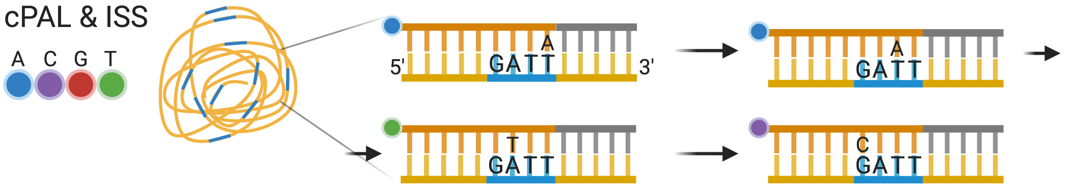
Figure 5.31: Schematic of cPAL as used in ISS.

The only in situ sequencing method that was reused after its inception was originally demonstrated in 2013 by Mats Nilsson’s group (Ke et al. 2013), which we call ISS here (Figure 4.7). First, padlock probes are hybridized to in situ reverse transcribed cDNAs and RCA amplified (Figure 5.18). The padlock probe can carry a gene specific 4 nt barcode (barcode version), or leave a 4 nt gap between the ends of the probe after it’s hybridized to the cDNA to be filled when the probe is circularized (gap filling version). Then the barcode or the filled gap is sequenced in situ, with an anchor primer binding 3’ to the target, with cPAL. Because of limited read length of cPAL, short sequences uniquely identify each gene and isoform for the gap filling approach becomes difficult to find with increasing number of genes and isoforms. In contrast, a barcode with length \(n\) can encode \(4^n\) genes and isoforms. As a result, the barcode approach was repeatedly used after the inception of ISS and was commercialized by CARTANA, which was recently acquired by 10X Genomics.

The barcode approach was initially used to profile 39 genes (Ke et al. 2013), but has been used to profile up to 222 genes in human brains affected by Alzheimer’s disease (W.-T. Chen et al. 2020). Although, as already mentioned, ISS has much lower detection efficiency than smFISH based methods, because of RCA and this low detection efficiency, the density of imaged amplicons is lower, allowing for imaging at lower resolution (20x; MERFISH uses 60x) and thus facilitating profiling large areas of tissues such as whole mouse brain coronal sections (Qian et al. 2020; Partel et al. 2019). ISS has also been used in conjunction with spatial transcriptomics techniques that are transcriptome wide but lack single cell resolution, such as ST. Panels of usually fewer than 100 genes of interest are selected from ST and scRNA-seq data, to be profiled with ISS for more in depth characterization of these genes (W.-T. Chen et al. 2020; Asp et al. 2019). In addition, because of the specificity conferred by the padlock probe and the small number of probes required per gene (usually 5 per gene but can be fewer), ISS has been used to quantify isoforms from isoform specific exons and exon-exon junctions (Lebrigand et al. 2020).

cPAL sequencing has also been used in BOLORAMIS (S. Liu et al. 2021) to profile transcripts of 96 genes and 77 miRNAs. Efficiency of padlock probe ligation when the template is RNA is improved with the SplintR ligase and careful placement of the ligation junction in the target region; the inefficiency of reverse transcription in ISS is avoided. With target sequence of 25 nt, shorter than that of STARmap (next section), BOLORAMIS has been adapted to target miRNAs that are 18-23 nt long, but barcode error rate for miRNAs is higher than that for mRNAs. While cPAL was used for demonstration, in principle, hybridization and SBS may be used to detect the barcodes. In terms of average number of spots per cell for 3 genes in BOLORAMIS vs. smFISH, efficiency of BOLORAMIS is 11% for GAPDH, 35% for POLR2A, and 12% for TFRC.

The number of genes that can be profiled by ISS is limited by the barcode length. Just like in seqFISH, only a small subset of all possible barcodes given a barcode length is used for error correction. As a result, to profile the entire transcriptome of over 20,000 genes, the barcode should be at least 8 nt long (65,536 barcodes), while in one direction, cPAL can only sequence 6 or 7 nt and degenerate bases. It is possible in theory to lengthen the barcode to up to 13 nt by sequencing from both ends of the barcode as in the original 2005 method (Shendure 2005). However, with increasing number of transcripts comes the problem of optical crowding, which is exacerbated by the physical size of the RCA amplicon. Perhaps ExM can be used here to mitigate optical crowding just like in ExSeq. To address the limitation in barcode length, HybISS, i.e. hybridization-based in situ sequencing, was devised (Gyllborg et al. 2020) so the now seqFISH-like barcode can be arbitrarily lengthened by increasing the number of rounds of hybridization. HybISS has already been reviewed in Section5.2.2.2; despite the “ISS” in its name, HybISS is classified as smFISH based because it does not involve SBL or SBS. HybISS also has up to 5 fold higher signal to noise ratio than ISS, and has somewhat higher detection efficiency than ISS though the improvement is less than 2 fold (average number of amplicons detected per cell for each channel in HybISS compared to ISS) (Gyllborg et al. 2020). Comparison between HybISS and smFISH has not been reported. Nevertheless, HybISS has not yet been scaled to more than 120 genes and ExM may still be needed for transcriptome wide profiling.

5.3.3 SEDAL and STARmap

Both SOLiD and cPAL have some drawbacks. As the gene specific barcode does not have to be long to encode all genes in the genome, when the barcode is used, limits in read length is not a major limitation. Because one color encodes two bases, SOLiD is very accurate (L. Liu et al. 2012), but error in one cycle propagates to later cycles. At least in the mouse brain, SOLiD also has high background (X. Wang et al. 2018). In contrast, cPAL does not have an inbuilt error rejection mechanism; the barcode must be elongated to allow for error correction, much like in the error correction scheme of seqFISH. Furthermore, in ISS, the mRNA is first reverse transcribed into cDNA because ligation of the padlock probe is inefficient when the template is RNA (Larsson et al. 2010). However, the efficiency of RT depends on the gene of interest and the variability of RT efficiency depends on RNA concentration (Schwaber, Andersen, and Nielsen 2019; Bustin et al. 2015).

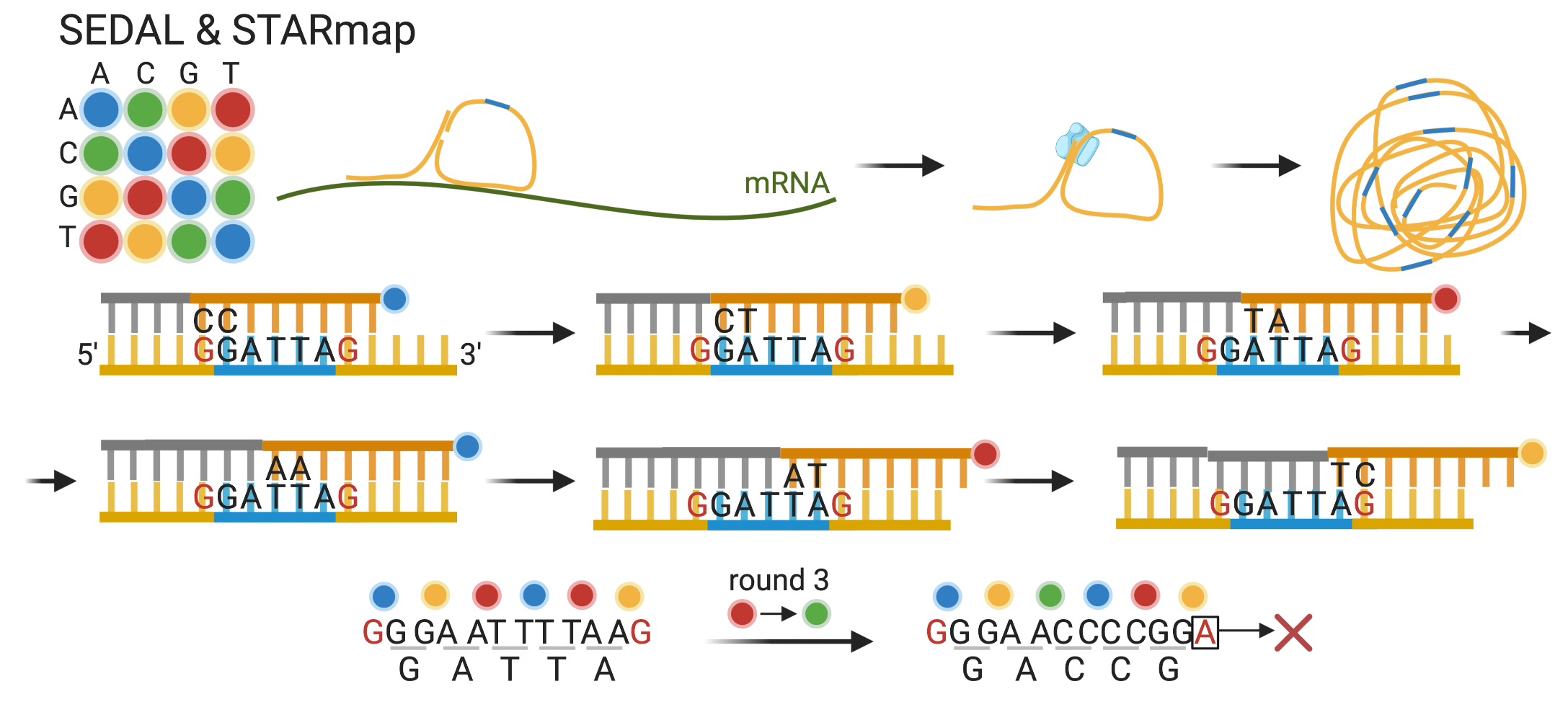
Schematic of RCA of SNAIL probe and SEDAL. Also showing error propagation and identification of 2 base encoding. As part of the constant region, the 'G' highlighted in red is known.

Figure 5.32: Schematic of RCA of SNAIL probe and SEDAL. Also showing error propagation and identification of 2 base encoding. As part of the constant region, the ‘G’ highlighted in red is known.

A new method of in situ sequencing, namely sequencing with error-reduction by dynamic annealing and ligation (SEDAL) in spatially-resolved transcript amplicon readout mapping (STARmap), was devised to address these shortcomings (X. Wang et al. 2018). In STARmap, the specific amplification of nucleic acids via intramolecular ligation (SNAIL) probe is a derivative of the original padlock probe that avoids RT altogether. A primer partially hybridizes to the mRNA, and partially to the padlock probe (Figure 5.32). The padlock probe carrying a 5 nt gene specific barcode hybridizes to the mRNA adjacent to the primer, but both ends of the padlock probe hybridize to the primer instead, so when the ends are ligated together, the template is DNA rather than RNA, thus avoiding both RT and inefficiency of ligation with RNA template, and then the primer is used to initiate RCA. As both the primer and the padlock probe must match the mRNA template for RCA to occur, SNAIL probes are specific and background of non-specific binding is eliminated. To reduce background autofluorescence and prevent the RCA amplicons from moving, the amplicons are crosslinked into a hydrogel and the tissue is cleared of proteins and lipids.

Then SEDAL is used to sequence the gene specific barcodes. The sequences flanking the gene barcode are known. In the first round an anchor or reading probe binds to the constant region 5’ to the barcode, one base away from the barcode (Figure 5.32). The decoding probes are 8-mers labeled with a fluorophore at the 5’ end whose color represents the 2 nucleotides at the 3’ end that interrogates the barcode; the other bases are degenerate. If the decoding probe matches the barcode, then it is ligated to the reading probe and the fluorescent signal is recorded. In the first round, the decoding probe interrogates the last base of the constant region and the first base of the barcode, as the last base of the constant region is necessary to decode the sequence of colors. Then the reading and decoding probes are stripped. In the second round, the reading probe stops right where the barcode starts. In the third round, the reading probe has a degenerate base extending into the barcode. Reading probes of the following rounds extend further into the barcode with degenerate bases. In the last round, the decoding probe interrogates the last base of the barcode and the first base of the following constant region. Like in SOLiD, with 2 base encoding, an error in a previous round propagates into later rounds; with propagation, when there is an error when decoding, then the first base of the constant region after the barcode would be incorrectly decoded, so the error is identified and rejected. Comparison of detection efficiency of STARmap with that of smFISH has not been reported; the efficiency is reported (average number of transcripts per cell for 151 cell type marker genes) to be somewhat better, at least not worse, than that of scRNA-seq, suggesting that STARmap is perhaps more efficient than ISS, but most likely much less efficient than MERFISH (HD4) and seqFISH.

5.3.4 Sequencing by synthesis

While most in situ sequencing techniques use SBL, some use SBS, indeed with a heated stage to perform SBS in situ. Because Illumina SBS is much more well-known and widely used than SBL for NGS, we will not recap it here. SBS has been tried to sequence DNA barcodes of antibodies in highly multiplexed immunofluorescence (Kohman and Church 2020). BARseq (X. Chen et al. 2019), a method to trace neuron projections is also based on SBS. In BARseq, the gap filling version of ISS (Section 5.3.2) is used and the filled gap that is the projection tracing barcode is sequenced with Illumina SBS chemistry. BARseq has also been adapted to profile endogenous transcripts (up to 79 genes as of writing) and image projection barcodes in the same neurons (BARseq2) (Y.-C. Sun et al. 2020; S. Chen et al. 2021); gene expression and projection can be correlated in some though not all cells. For endogenous transcripts, the mRNA is first reverse transcribed, and the barcode version of ISS (Section 5.3.2) is used to amplify the barcodes (in the padlock probe but not the cDNA) with RCA, which are then sequenced in situ with SBS. For transcripts, BARseq2 detects slightly more copies of mRNAs than 10X v3 scRNA-seq for the same gene in the same tissue.

5.4 NGS with spatial barcoding

This section reviews techniques that capture transcripts from a permeabilized tissue section on a spatially organized array for RNA-seq. These techniques are similar to 3’ based scRNA-seq, with amplification and sequencing handle, barcode, UMI, and poly-T to capture polyadenylated transcripts, except that each spot in the array has its own barcode, rather than each droplet. As the spots are not organized in a regular array in Slide-seq, PIXEL-seq, and Seq-scope, this section more generally concerns techniques that pre-determine spatial locations of each spatial barcode before capturing polyadenylated transcripts, so the spatial location is encoded by the barcode rather than selection and isolation of ROIs. These techniques are generally transcriptome wide, but do not have single cell resolution; the resolution is the size and shape of the spots and spacing between the spots. In ST and Visium, the array is constructed by printing the capture sequences onto commercial microarray slides, so the 5’ end of the sequences are attached to the slide; where each spatial barcode is placed is known. In DBiT-seq, the array is constructed by depositing barcodes specific to each microfluidic channel with orthogonal channels. Alternatively, the capture sequences can be attached to beads like in droplet scRNA-seq, as in Slide-seq and HDST. The beads are randomly placed on a slide in a single layer, and the location of barcodes are determined before library preparation when the capture sequences and transcripts are released from the slide.

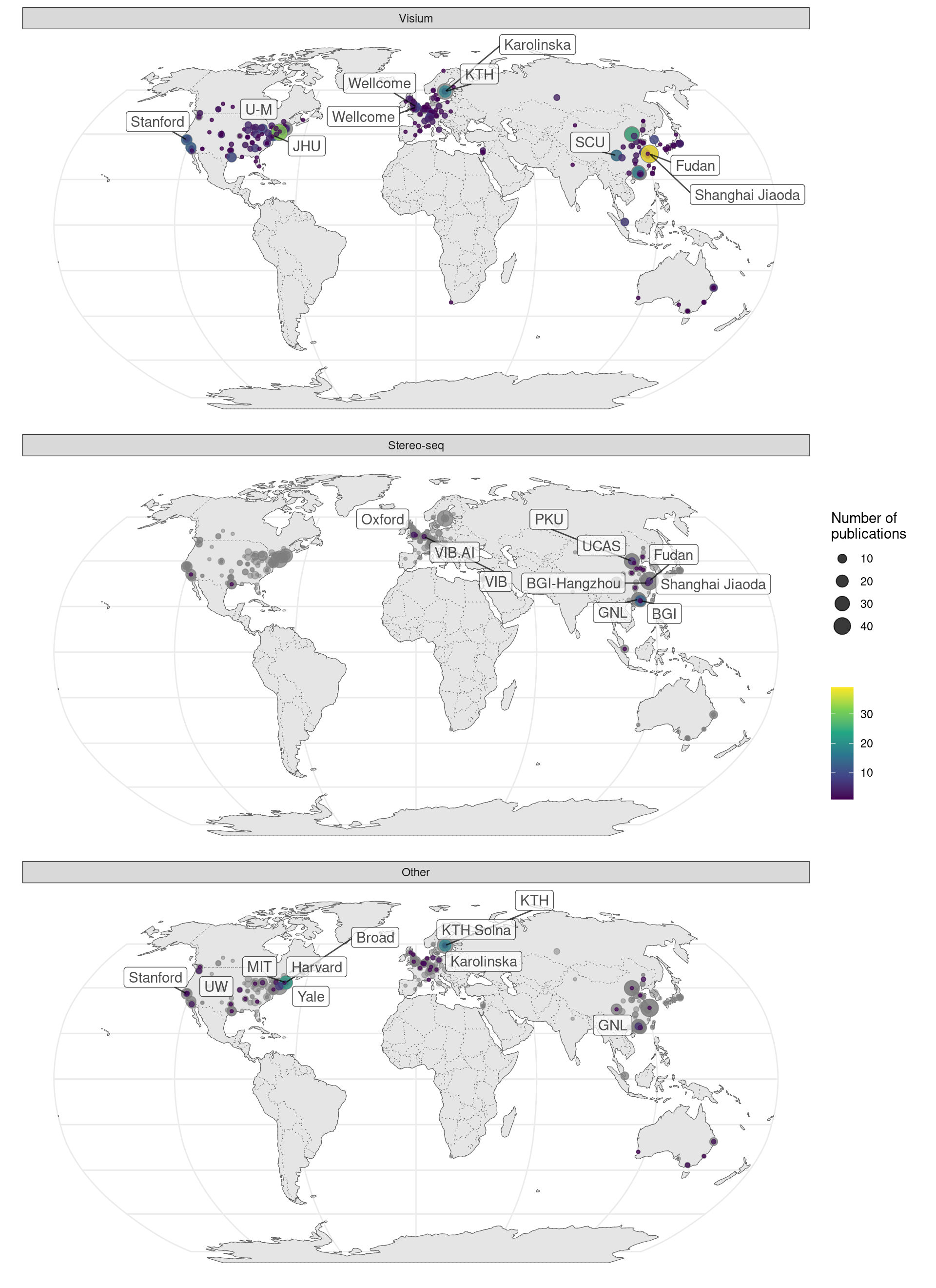
Cities and institutions using the two most popular technologies worldwide, the two methods used by the most institutions. Preprints are included.

Figure 5.33: Cities and institutions using the two most popular technologies worldwide, the two methods used by the most institutions. Preprints are included.

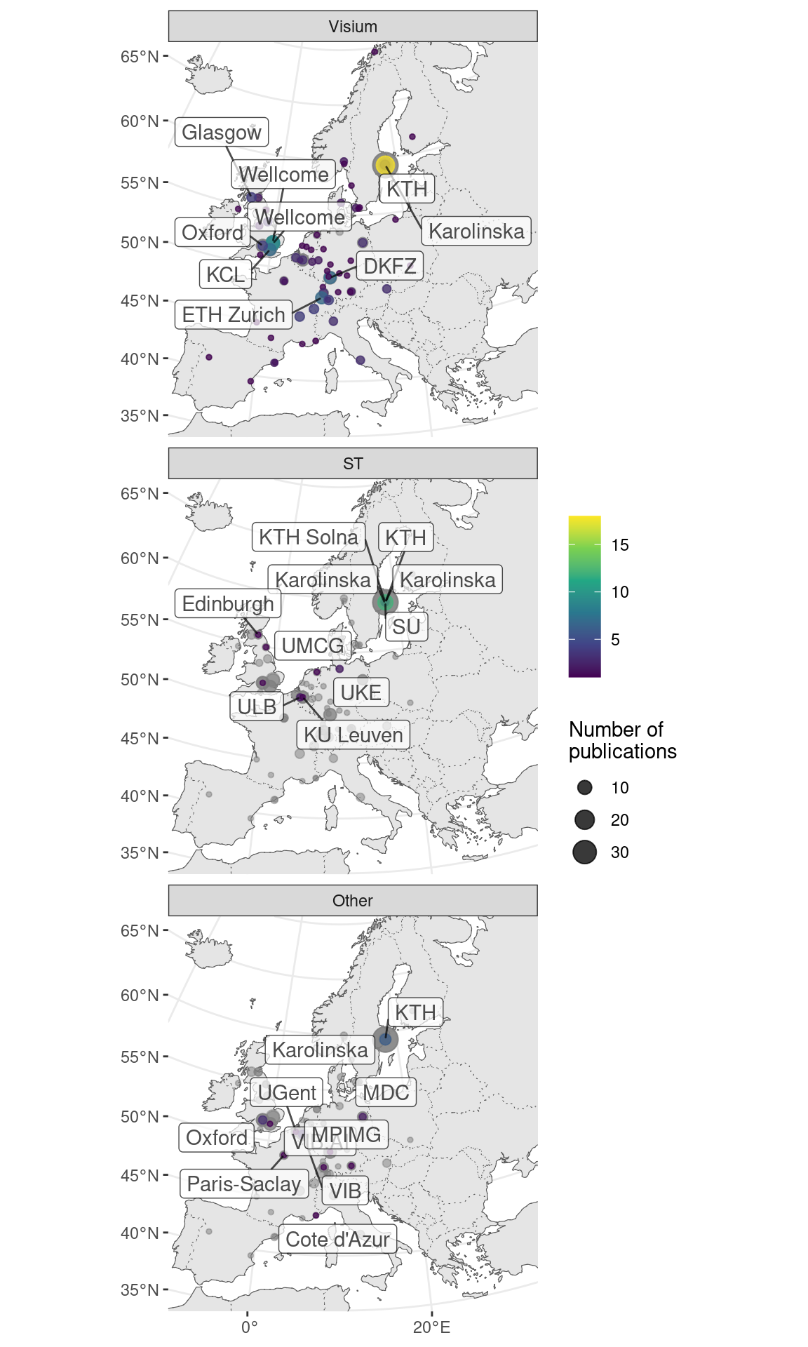
Figure 5.34: Cities and institutions using the two most popular tehcnologies in western Europe. Preprints are included.

ST (Ståhl et al. 2016) and Visium are the most widely used NGS barcoding based techniques worldwide (Figure 4.7, Figure 5.33). In ST, the printed spots have diameter of 100 \(\mu\)m and are 200 \(\mu\)m apart from center to center (Figure 5.35). Multiple sections can be mounted to the same slide, separated by a rubber mask. For each section, there are 1007 spots covering an area of 6200 \(\times\) 6600 \(\mu\)m. The 5’ end of the capture sequence is a linker to be cleaved to release the transcripts, followed by amplification and sequencing handle, an 18 nt spatial barcode, a 9 nt UMI, and poly-T (Figure 5.36). For the genes quantified with smFISH, ST’s detection efficiency is around 6.9% compared to smFISH (transcript count per area for 3 genes in corresponding regions in adjacent sections), within the range of the efficiency of scRNA-seq techniques. Despite the low resolution, ST is popular probably due to transcriptome wide profiling, ease to apply to larger area of tissue, not requiring specialized equipment such as SRM and custom fluidics systems, commercial kits, possible automation of library preparation (Jemt et al. 2016), availability of a documented and open source data preprocessing pipeline called ST Pipeline (Navarro et al. 2017), and the extra information from H&E staining before library preparation.

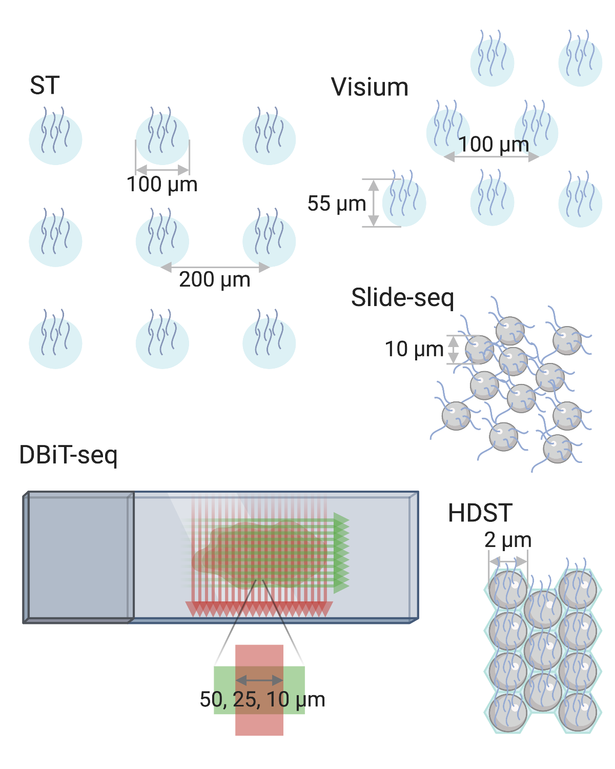
Figure 5.35: Schematic of spot construction and size of array based techniques.

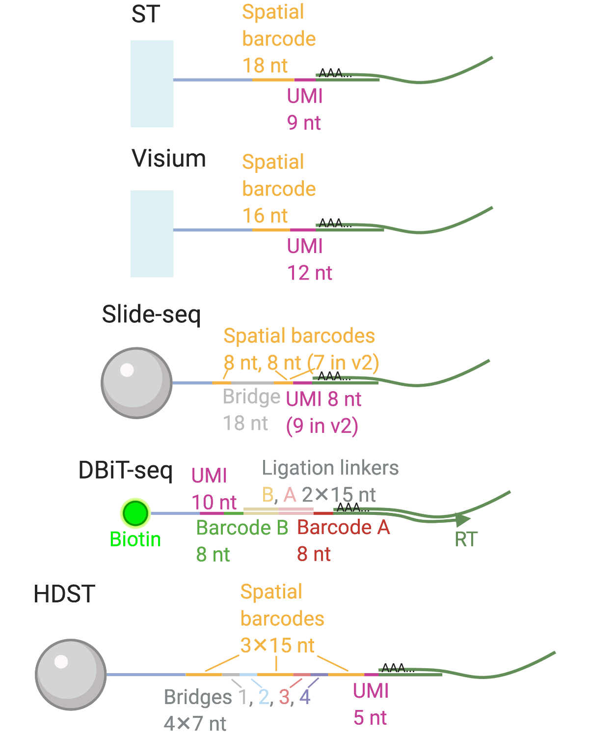
Figure 5.36: Barcode and UMI structure and lengths of array based techniques.

After its inception, ST has been used in a wide range of clinical pathological tissues, such as heart after heart failure (Asp et al. 2017), peritonitis-affected gingival tissue (Lundmark et al. 2018), prostate cancer (Berglund et al. 2018), breast cancer (He et al. 2020), arthritic joint biopsies (Carlberg et al. 2019), lymph nodes affected by melanoma metastasis (Thrane et al. 2018), spinal cords (Maniatis et al. 2019) and cerebellums (Gregory et al. 2020) affected by amyotrophic lateral sclerosis (ALS), and squamous cell carcinoma (A. L. Ji et al. 2020). ST has also been used to construct gene expression atlases of healthy tissues such as the developing human heart (Asp et al. 2019) and the mouse brain (Ortiz et al. 2020). Common downstream data analyses include identifying differentially expressed (DE) genes between diseased and healthy regions, gene set enrichment analysis (GSEA) among DE genes, and cell type deconvolution of the spots by integrating ST and scRNA-seq data. Data analysis methods designed specifically for ST or Visium will be reviewed in more detail in Chapter 7.

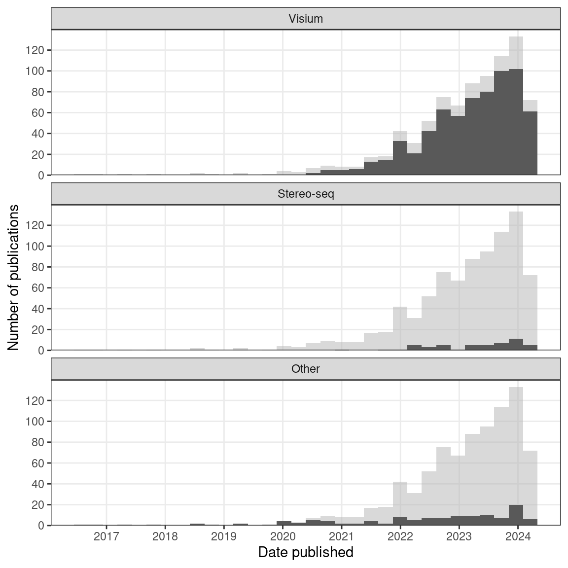
Figure 5.37: Number of publications over time, broken down by technique. The facets are ordered by total usage of the technique. Bin width is 90 days.

After 10X Genomics acquired ST in December 2018, the succeeding 10X Visium has quickly gained popularity and spread far and wide (Figure 4.7). Visium has superseded ST and has become the most popular current era technology (Figure 5.33, Figure 5.37). While ST is still the second most popular NGS barcoding technology in Europe (Figure 5.34), it seems concentrated in Sweden, where ST comes from. In contrast, usage of Visium is more decentralized (Figure 5.33). Visium is similar to ST and shares the advantages of ST, but with higher spatial resolution. The spots are 100 \(\mu\)m apart center to center, each with a diameter of 55 \(\mu\)m, arranged in a hexagonal configuration (Figure 5.35). After adjusting for spot area, Visium seems to capture somewhat more transcripts and genes compared to ST (Y. Liu, Yang, et al. 2020), but more datasets in the same tissues and accounting for sequencing depths are needed to make a fairer comparison. In addition, Visium’s growth in popularity may be due to core facilities at multiple institutions providing Visium services (“10X VISIUM SPATIAL TRANSCRIPTOMICS,” n.d.; “ADVANCED GENOMICS CORE PRICING,” n.d.; “SpaRTAN,” n.d.). As a new version of ST, Visium was originally designed for fresh frozen OCT embedded tissue and 3’ Illumina sequencing. However, Visium has more recently been adapted to FFPE tissue (Villacampa et al. 2020) (the now commercial Visium FFPE has a very different chemistry from (Villacampa et al. 2020)), as well as to Nanopore long read sequencing to quantify isoforms (Lebrigand et al. 2020; Joglekar et al. 2020), although Visium is still predominantly used on fresh frozen tissues for 3’ end sequencing.

Visium studies in our database are almost exclusively on humans and mice, and mostly on humans (Figure 5.38). For a long time, in both humans and mice, and both the healthy and pathological cases, the brain is again the most studied organ (Figures 5.39, 5.40), but more studies have been performed on other organs in humans more recently. This is in stark contrast with usage of GeoMX DSP, which was used in several COVID lung studies but not much in brain (Figure 5.9).

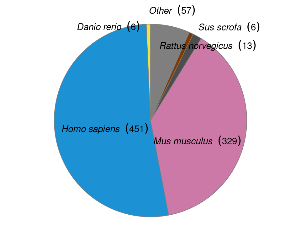
Figure 5.38: Number of publication per species.

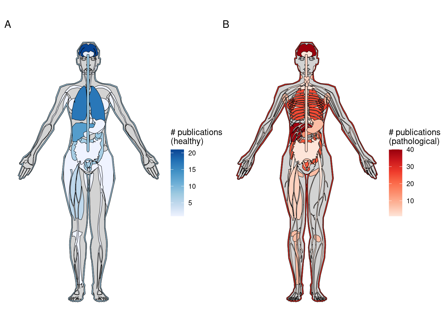
Number of Visium studies for healthy (A) and pathological (B) human organs. Female is shown here due to several breast cancer and ovary studies. There is one human prostate Visium study in our database (McCray et al. 2021).

Figure 5.39: Number of Visium studies for healthy (A) and pathological (B) human organs. Female is shown here due to several breast cancer and ovary studies. There is one human prostate Visium study in our database (McCray et al. 2021).

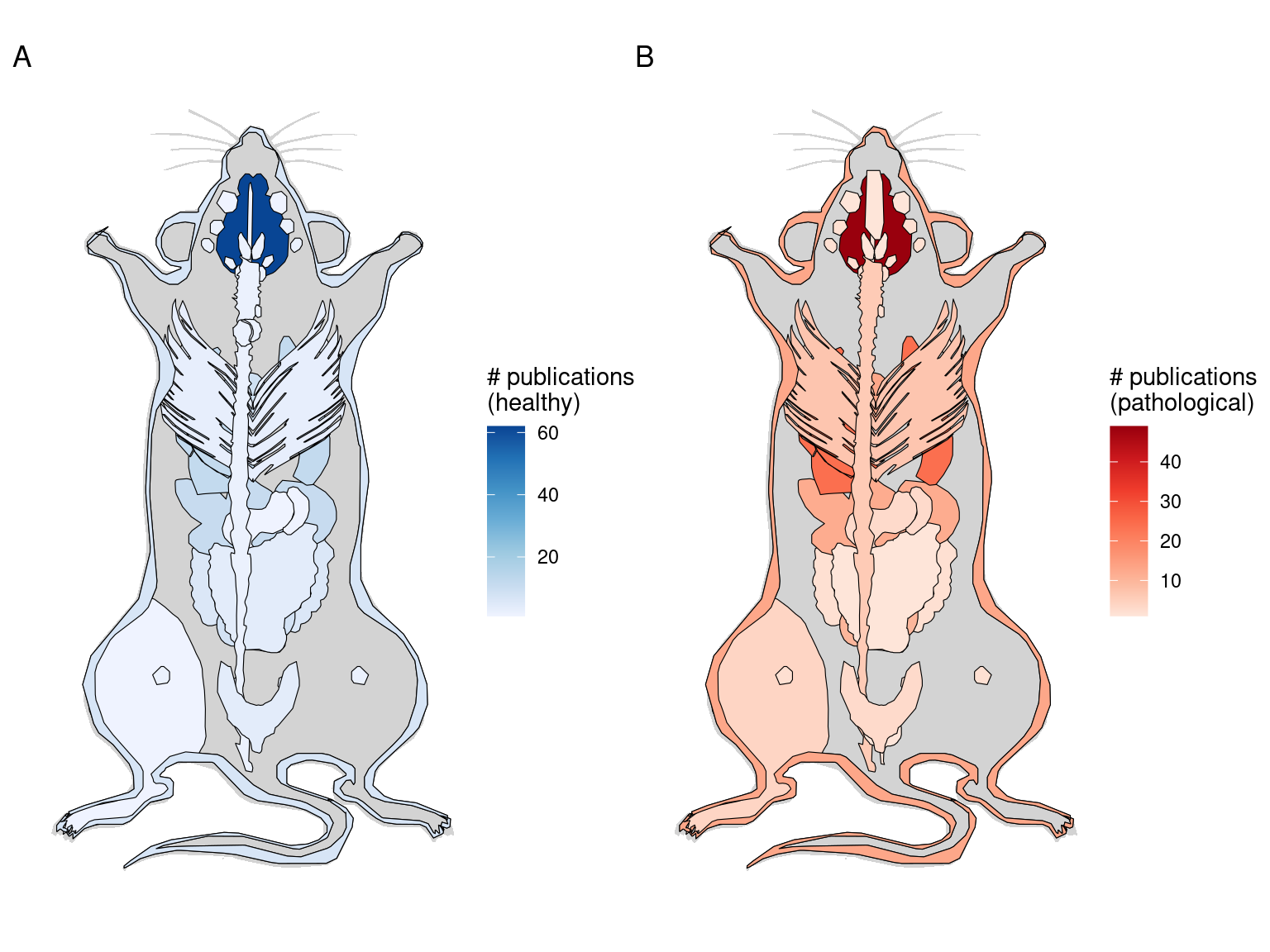
Number of Visium studies for healthy (A) and pathological (B) mouse organs. Female is shown here as there is a uterus study while there is no study on male specific organs in our database.

Figure 5.40: Number of Visium studies for healthy (A) and pathological (B) mouse organs. Female is shown here as there is a uterus study while there is no study on male specific organs in our database.

In response to the low resolution of ST, Slide-seq was developed to increase the resolution of array based spatial transcriptomics (Rodriques et al. 2019). Beads like those used in Drop-seq (Macosko et al. 2015) with diameter 10 \(\mu\)m are spread on a slide in a single layer, not necessarily in a regular grid, and bead barcodes are generated with 16 rounds of split pool, each round adding one nucleotide, broken into 2 blocks of 8 nt (2 blocks of 8 and 7 nt in version 2) (Figure 5.35, Figure 5.36). As the location of each barcode is not pre-determined, the slide is imaged and the barcodes are sequenced in situ with SOLiD. Then the OCT frozen tissue section is mounted on the layer of beads on the slide and the beads are removed for library preparation. The first version of Slide-seq is very inefficient; for the genes compared, the Slide-seq only detects 2 to 3 orders of magnitude fewer transcripts per cell for 3 genes than smFISH in an adjacent section and about 2.7% compared to Drop-seq for the same cell type from CA1 (Rodriques et al. 2019).

In the second version of Slide-seq (Slide-seq2) (Stickels et al. 2020), the barcodes are sequenced by SEDAL (like in Figure 5.32, but with one color per base) rather than SOLiD, which increased the efficiency of spatial mapping of Illumina reads, probably because of error propagation in the 2 base encoding of SOLiD. Moreover, bead synthesis is further optimized and a second strand synthesis step is added to the library preparation to increase the number of cDNAs for PCR amplification. Efficiency is improved in Slide-seq2, which is ~9.3x higher than version 1, about on par with Drop-seq, 1 order of magnitude lower than that of smFISH, and somewhat better than Visium in the dataset chosen. Here “efficiency” means number of UMIs or transcripts for 3 genes from a fixed area in CA1. The official software to process the in situ sequencing images is written in MATLAB, which is proprietary. Although the size of the bead is close to the size of a single cell, Slide-seq does not have single cell resolution as one bead can capture transcripts from more than one cells nearby, so cell type deconvolution of beads is still needed. After its inception, Slide-seq2 has been used on mouse and human testes, at the institution of origin (W.-T. Chen et al. 2020).

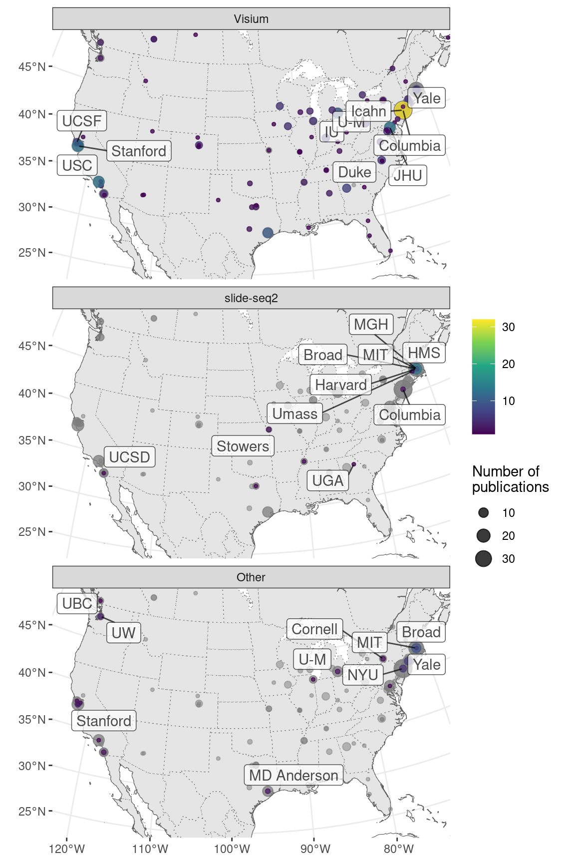
Figure 5.41: Cities and institutions using the two most popular technologies around continental US. Preprints are included.

Slide-seq is the second most popular NGS barcoding technique around the US, but unlike Visium (the most popular), Slide-seq is still more concentrated around Broad, Harvard, and MIT, where it was first developed (Figure 5.41).

Spatial resolution of array based techniques has been further increased with HDST, with a resolution of 2 \(\mu\)m (Vickovic et al. 2019), which is smaller than a single cell. Like in Slide-seq, beads like those used in droplet scRNA-seq are used. The diameter of each bead is 2 \(\mu\)m, and hexagonal wells with diameter 2.05 \(\mu\)m are carved into a slides so each well contains one bead (Figure 5.35). The spatial barcodes are generated by 3 rounds of split-pool, each round adding 15 nt from the barcode pool (Figure 5.36). The UMI is only 5 nt but such a small area does not contain that many transcripts. As the beads are randomly placed in the wells, the locations of barcodes need to be determined. Four rounds of FISH, with combinations of red, green, and no color, encode each of the 3 barcodes on each bead. Again, HDST was originally designed for fresh frozen OCT embedded tissue rather than FFPE. HDST is very inefficient; for the genes compared, the detection efficiency is only ~1.3% compared to smFISH per bead area. To our best knowledge, HDST has not been used for new datasets after its inception.

In response to the low efficiency and complicated procedure to localize barcodes of Slide-seq and HDST, Deterministic Barcoding in Tissue for spatial omics sequencing (DBiT-seq) was developed, with resolution up to 10 \(\mu\)m (Y. Liu, Yang, et al. 2020). Let \(i, j\) denote the index of channel in each direction. Barcode \(A_i\), attached to poly-T, is flown across the slide in microfluidic channels and RT is performed (Figure 5.35). Then barcode \(B_j\), attached to the UMI, PCR handle, and biotin, is flown across the slide in microfluidic channels perpendicular to those that delivered barcode \(A_i\), and barcode \(B_j\) is ligated to barcode \(A_i\) and the cDNA (Figure 5.35, Figure 5.36). Then the ligated barcodes and cDNA can be purified by streptavidin-coated magnetic beads. Each microfluidic channel carries a different barcode, so where the channels for barcodes \(A_i\) and \(B_j\) intersect, an array is created and the location of each spot is encoded by \(i, j\). The resolution is limited by the width of the channels and the spacing between them; widths of 50, 25, and 10 \(\mu\)m have been tested. Per unit spot area, DBiT-seq seems to detect at least 3 times more genes and UMIs than ST and Visium and the improvement is even starker at the 10 \(\mu\)m resolution. For the genes compared, DBiT-seq’s detection efficiency is ~15.5% of that of smFISH per unit area, making it relative more sensitive among the array based methods reviewed here. DBiT-seq has also been adapted to FFPE, although just like in Visium, RNAs in FFPE tissues are more degraded than in fresh frozen tissues and fewer genes and UMIs are detected per unit area in comparable tissue types (Y. Liu, Enninful, et al. 2020).

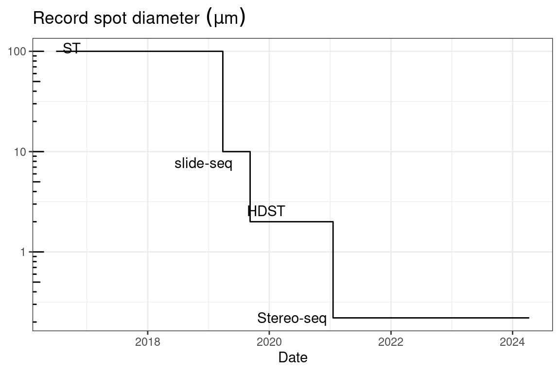
Figure 5.42: Record spot diameter of array based methods over time.

The record resolution of array based techniques is ever increasing (Figure 5.42); sub-micron techniques are appearing in 2021. The record is broken by Stereo-seq in January 2021, reporting a spot diameter of 220 nm although the distance between spots is 500 or 715 nm (A. Chen et al. 2021). In Stereo-seq, circularized DNA containing a random 25 nt barcode is RCA amplified and deposited into an etched grid. The barcode is sequenced and then oligos with polyT and molecular ID are hybridized to the barcode to capture polyA transcripts from the mounted tissue. The reported capture efficiency is around 170 UMIs per 100 \(\mu m^2\) in mouse brain, on par with that of the Visium mouse brain dataset from the 10X website reanalyzed in the same study.

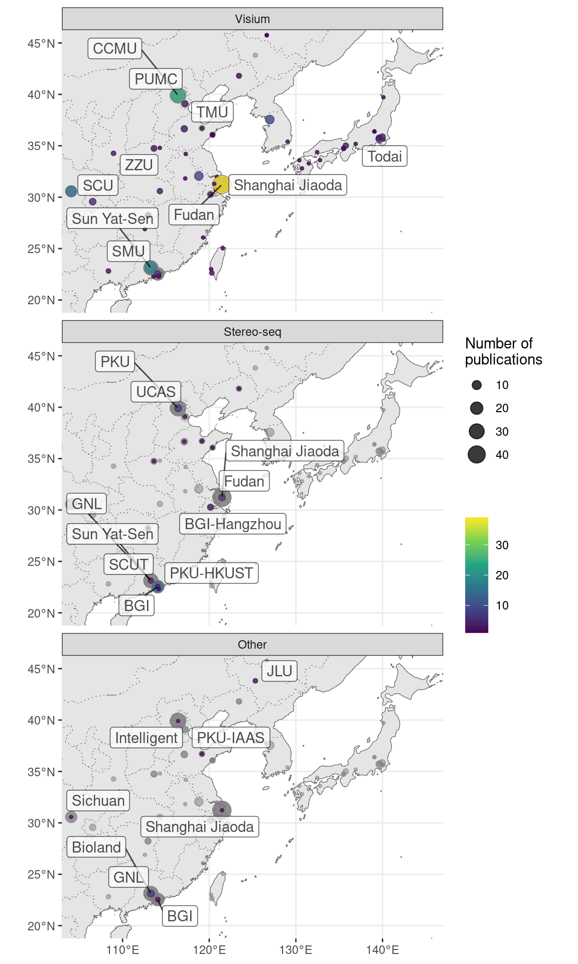
Figure 5.43: Cities and institutions using the two most popular tehcnologies in Northeast Asia. Preprints are included.

In Northeast Asia, Visium is the most popular method and is used in many less well-known institutions across different countries. The second most popular technology is Stereo-seq, which has been commercialized by BGI, although its use is concentrated around BGI Shenzhen where it was developed (Figure 5.43).

Another sub-micron array capture method is Seq-Scope (Cho et al. 2021), which creates clusters of polyT capture sequences each with its own spatial barcode (20-32 nt) from Illumina bridge amplification on a repurposed Illumina flow cell. The spatial barcode is sequenced with SBS. Then the flow cell is dismantled so the tissue can be mounted for transcript capture. The captured transcripts are then sequenced with NGS. The clusters can have a diameter down to 0.5 \(\mu\)m, and the clusters are randomly seeded, not distributed in a grid. The reported capture efficiency is around 1000 and up to 2000 UMIs per 100 \(\mu m^2\) in mouse colon, much higher than that of Stereo-seq, although we are not sure whether colon data is comparable to brain data here.

A more recent nearly sub-micron technique is PIXEL-seq (Fu et al. 2021). Again, as in the Illumina flow cell, PIXEL-seq amplifies each randomly seeded spatial barcode (24 nt) and polyT capture sequence into polonies. However, here a crosslinked polyacrylamide gel (rather than a linear one in Illumina) is used, to form continuous polonies without much space between their “territories” rather than discrete clusters. The spatial barcodes are also first sequenced with SBS before the tissue is mounted for transcript capture. On average, the polony is around 1.17 \(\mu m^2\) in area, so assuming it is circular, then the diameter is 1.22 \(\mu\)m. The reported capture efficiency is around 1000 UMIs per \(\mu m^2\) in mouse brain, which might be comparable to that of Seq-Scope.

While such sub-micron techniques have subcellular resolution, in practice, the data is binned into much larger grids for standard scRNA-seq analysis, such as \(36\mu m\times36\mu m\) in Stereo-seq and \(10\mu m\times10\mu m\) or \(7\mu m\times7\mu m\) or \(5\mu m\times5\mu m\) in Seq-Scope. The subcelluar information was not directly used in the analyses, although even with binning, the resolution is still higher than that of ST and Visium.

All these array and NGS based techniques reviewed so far capture polyadenylated transcripts. While miRNAs form a major topic in LCM literature (Figure 6.3) and are profiled in some prequel era ISH atlases, current era techniques mostly preclude miRNA quantification. BOLORAMIS has been demonstrated on 77 miRNAs, but the barcode error rate is higher than in mRNAs. Without a poly-A tail, miRNAs are precluded by NGS based techniques that rely on poly-A capture. To quantify miRNAs in space, an array based technique was developed as an alternative to LCM and designed for FFPE tissues (Nagarajan et al. 2020). The tissue is pixelated, and each pixel is 300 \(\mu\)m \(\times\) 300 \(\mu\)m. Within each pixel is a smaller 3 \(\times\) 3 array, each spot of which has probes for one miRNA; The locations of the spots within each pixel can be easily discerned with a fluorescent microscope. This way, up to 9 miRNAs can be profiled in the same tissue section at the same time, although the 9 miRNAs are from somewhat nearby cells but not the same cells.

5.4.1 Gray areas and single cell resolution

In Section 5.1.4, the definition of “microdissection” is relaxed, so that cell sorting can be some kind of “microdissection”, and GeoMX DSP is described there because like most microdissection methods, it’s primarily used for targeted ROIs rather than regular grids and spatial location is known from selection of the ROI. Due to the fuzziness of “microdissection”, some techniques that assign spatial barcodes to a regular grid but dissociate each spot in the array into single cells may or may not be considered de facto “microdissection”. Because of the regular grid as in Visium and DBiT-seq and that spatial location is known by pre-determined spot barcode rather than selection of ROI, these techniques are summarized in this section.

In Visium, all cells within the same spot get the same spot barcode, so the transcriptome of each spot is from mixture of different cells, often different cell types. Cell types can be computationally deconvolved with software such as Stereoscope (Alma Andersson et al. 2020) and CIBERSORT (Newman et al. 2015) with a reference of transcriptomes of known cell types. To address this problem, some new array capture spatial techniques impart each spot a spatial barcode before the cells or nuclei in the spots are dissociated and assigned another cell specific barcode for scRNA-seq, so the transcriptomes have single cell resolution, though not single cell spatial resolution as the location of each cell within the spot is not recorded and the spatial resolution is lower than that of Visium. In XYZeq (Y. Lee et al. 2021), spot barcodes with UMIs and poly-T capture sequences are deposited in microwells 500 \(\mu\)m center to center arranged in an array. The tissue sections is fixed with dithio-bis(succinimidyl propionate), which preserves RNA integrity for scRNA-seq. The tissue is permeablized and incubated in an microarray hybridization chamber for the spatial barcodes to hybridize to polyadenylated transcripts and for reverse transcription, so the cDNA acquires the spatial barcode. Then the cells are sorted into PCR wells and the cell barcode is added from a PCR primer. A related method is sci-Space (Srivatsan et al. 2021), where spatial “hashing” oligos are spotted in a an array on a slide covered with dried agarose. The spots are on average about 73.2 \(\mu\)m in radius and about 222 \(\mu\)m apart center to center. The hashing oligos diffuse into the nuclei in the tissue mounted on the slide, and the spatially hashed nuclei are dissociated for sci-RNA-seq.

5.5 Detection efficiencies

In the previous few sections we have mentioned detection efficiency many times. To recap, these are common methods to estimate detection efficiency of spatial transcriptomics techniques:

Gold standard smFISH and the single molecule resolution technique of interest are performed in the same cells for a small number of genes and the numbers of transcripts spots detected in each segmented cell from smFISH and the technique of interest are compared. This was performed for HCR-seqFISH and ExSeq.
Gold standard smFISH and the single molecule resolution technique of interest are performed on different cells of the same type or on adjacent sections for a relatively small number of genes. Then average transcript counts of each gene per cell among these cells are compared between smFISH and the technique of interest. This was performed for MERFISH and seqFISH+, and was used to compare efficiencies of HybISS and HybRISS (H. Lee et al. 2020).
Gold standard smFISH is performed on an adjacent section for a small number of genes. Transcript spot counts from smFISH and UMI counts from the NGS based technique per unit area in the same tissue type are compared. The unit area can have the same shape and size of the transcript capture spot, or can contain multiple spots and averaged over the spots. This was performed for ST, HDST, and Slide-seq(2).
UMI or transcript spot counts of select marker genes per cell in the spatial techniques of interest are compared to those in scRNA-seq of the same cell type. This was performed for STARmap and Slide-seq(2). In Slide-seq(2), as the tissue section is imaged, nuclei can be segmented and counted so the number of cells in the ROI compared is known and an equivalent number of cells from scRNA-seq is sampled for comparison.
Number of all UMI and genes detected per unit area in one NGS based spatial technique is compared to those of other NGS based spatial techniques. This was performed for DBiT-seq, Visium (FFPE), Stereo-seq, PIXEL-seq, and Seq-Scope. A caveat is that sequencing depth is not always considered.
The number of reads per cell is compared between scRNA-seq and FISSEQ. This is only known to be performed for FISSEQ.

In summary, a putative ranking, from high to low, of capture efficiencies of current era techniques, noting which methods above are used to estimate the efficiencies, is:

smFISH (~100%) > MERFISH (2, HD4, ~95%) > HCR-seqFISH (1, ~86%) > ExSeq (1, targeted, 62%) > seqFISH+ (2, ~49%) > (maybe) Seq-Scope (5) ~ PIXEL-seq (5) > (maybe) DBiT-seq (3, 5, ~15%) ~ Visium ~ Stereo-seq (5) > (maybe) HybRISS (2 with HybISS) > HybISS (2 with ISS and HybRISS) ~ (maybe) STARmap (4) ~ (maybe) scRNA-seq ~ Slide-seq2 (3, 4) ~ ST (3, ~6.9%) ~ ISS (~5%) > HDST (3, ~1.3%) > Slide-seq1 (3, 4, ~1%) > FISSEQ (6, 0.005%)

A percentage is not shown where it is not reported. This is putative because this is based on reports in the main text. There are conflicting reports of capture efficiency of Visium and DBiT-seq. Furthermore, comparison of different tissues and different genes from those studies may be problematic. For some of the technologies, the capture efficiency is compared to that of smFISH with only a few genes. Multiple datasets from each technology for as similar a tissue as possible for the same set of genes should be compared to get a better idea about the capture efficiency of each technique. Moreover, other factors such as tissue handling, sequencing depth, and data processing software may influence the results.

While fresh frozen tissues are predominantly used in the current era, DBiT-seq, Visium, and LCM have been adapted to FFPE tissues. RNAscope can be used on FFPE tissue for up to 12 targets. GeoMX DSP has been predominantly used on FFPE tissues. FFPE is a common way to archive tissue specimen, and sometimes the only tissues available is FFPE, sometimes years if not decades old. From techniques that have both fresh frozen and FFPE protocols, FFPE and storage of FFPE samples seem to significantly degrade the transcripts and reduce detection efficiency, but there can still be enough information preserved to identify cell types in the spots and correlation between gene expression measured in FFPE and fresh frozen tissues is usually high. In the pre-commercial FFPE Visium mouse brain dataset from the protocol of (Villacampa et al. 2020), at a sequencing depth of ~50,000 reads per tissue covered spot, the spots have on average ~1200 genes and ~2200 UMIs detected. In contrast, in a similar fresh frozen mouse brain section, with sequencing depth of ~115,000 reads per tissue covered spot, the spots have on average ~6000 genes and ~27200 UMIs detected. While the fresh frozen sample has higher sequencing depth, FFPE seems to reduce the number of genes and UMIs detected beyond the impact of sequencing depth. As Visium captures the transcripts on spots printed to a glass slide, the transcripts need to be dissociated from the tissue, and in the case of FFPE, it means de-crosslinking. However, commercial FFPE Visium today has a very difference chemistry from (Villacampa et al. 2020) and is said to be much more efficient. In FFPE DBiT-seq, the transcripts don’t have to be de-crosslinked as the barcodes are deposited into the tissue. FFPE reduced cDNA length from an average of ~1400 nt in PFA fixed fresh frozen tissue to about ~600 nt on average. In mouse embryos, while DBiT-seq on PFA fixed fresh frozen tissue gives on average 2100 genes and 4688 UMIs per 25 \(\mu\)m spot, FFPE tissue gives only 355 genes and 520 UMIs in the same sized spots on average (Y. Liu, Enninful, et al. 2020). However, sequencing depth is not discussed. From these studies, in both Visium and DBiT-seq, FFPE might decrease detection efficiency in terms of number of UMIs detected per unit area by about 5 (if considering sequencing depth in the Visium study) to 10 folds.

5.6 De novo reconstruction of spatial locations

The techniques reviewed above, involve either imaging (e.g. LCM, smFISH, ISS, Slide-seq, and HDST) or prior knowledge of locations (e.g. Tomo-seq, ST, Visium, and DBiT-seq). Some spatial transcriptomics techniques have been developed that require neither imaging nor prior knowledge of locations, and we review these in this section. While techniques that deposit spatial barcodes in an array at known locations such as Visium and DBiT-seq do not require imaging to know the location of gene expression, the spatial barcode locations are known a priori. In contrast, techniques reviewed in this section do not involve a priori knowledge of locations.

It is possible to reconstruct relative locations of cells or transcripts from colocalization without imaging, albeit imperfectly. These techniques are reviewed in more details in (Boulgakov, Ellington, and Marcotte 2020); we will only briefly summarize techniques that do not require DNA bound to a surface so they can be applied in cells and tissues. An early method to do so is Puzzle Imaging, published in 2015 (Glaser et al. 2015). Here “colocalization” can mean whether two neurons have axons in the same voxel or whether two neurons are synaptically connected. The spatial reconstruction is framed as a dimension reduction problem; each voxel is represented as a vector with \(n\) dimensions, where \(n\) stands for the number of neurons, and these vectors are to be projected into 2 or 3 dimensions, representing spatial dimensions, for reconstruction. Puzzle Imaging was only demonstrated in synthetic datasets, but not real biological datasets. Such reconstruction was made possible for transcripts with DNA microscopy (Weinstein, Regev, and Zhang 2019; Hoffecker et al. 2019). Transcripts are reverse transcribed in situ, and the cDNA, with an UMI added, is PCR amplified in situ. The amplified products diffuse and encounter amplified products from other transcripts. The nearby cDNAs are concatenated with overlap extension PCR, with additional random sequences in the overlapping primers to encode each concatenation event, called unique event identifier (UEI). When the concatenated cDNAs are sequenced, the two UMIs and the UEI are recorded. Because amplified products from two nearby transcripts are more likely to be concatenated than those from two transcripts that are far apart, the number of UEIs between two UMIs can be used to reconstruct relative distance between transcripts.

Techniques have also been developed to quantify transcripts from subcellular compartments, such as APEX-RIP (Kaewsapsak et al. 2017) and APEX-seq (Fazal et al. 2019). Although these techniques do not record or reconstruct spatial coordinates, they are included in this review because the publications describing them described them with terms such as “spatial”, “localization”, and “spatial transcriptome”. APEX is an engineered ascorbate peroxidase, which can be targeted to specific cellular compartments by expressing a fusion of APEX and a protein targeted to the compartment of interest. With substrates H₂O₂ and biotin-phenol (BP), APEX catalyzes formation of biotin-phenoxyl radicals that can biotinylate nearby proteins, which can be isolated with streptavidin. In APEX-RIP, mRNAs are cross linked to nearby proteins and thus isolated after isolating biotinylated proteins. In contrast, in APEX-seq, the mRNAs are directly biotinylated. Compared to APEX-RIP, APEX-seq better discerns transcript localization in compartments not bound by membrane. However, both APEX-RIP and APEX-seq were originally designed for bulk rather than single cell samples and was tested only on cell culture. Also, because a fusion protein is required, they cannot be performed in human tissue sections.

Rare cell types are difficult to characterize with most spatial transcriptomics techniques. ST and Visium lack single cell resolution and signal from rare cell types may be diluted by signal from common cell types in the same spot. LCM is still typically not used on single cells and rare cell types may or may not be easily discernible with H&E. SmFISH based techniques and targeted ISS require a pre-defined panel of genes, often selected from scRNA-seq and well-known markers, but such selection is more challenging for rare cell types, which may not be well-studied enough to begin with due to challenges in other transcriptomics techniques. However, spatial pattern of genes expressed in rare cell types can be characterized by deliberately creating doublets or multiplets involving both common and rare cell types, as in paired cell sequencing (Halpern et al. 2018) and ClumpSeq (Manco et al. 2020). Earlier, RNA-seq has been performed to cell multiplets to identify physical interactions between cell types in the mouse bone marrow in ProximID, but reconstruction of spatial locations was not attempted (Boisset et al. 2018). Spatial patterns of genes expressed in common cell types such as hepatocytes and small intestine enterocytes are already known from smFISH or LCM and spatial reconstruction of scRNA-seq data (Halpern et al. 2017; Moor et al. 2018). Genes expressed in the rare cell types are identified from genes much more highly expressed in the multiplet than in individual cells from common cell types in scRNA-seq, or markers of rare cell types from scRNA-seq if such data exists. Then the multiplets are mapped to spatial locations with patterned genes expressed by common cell types and existing smFISH or LCM data as reference. Then rare cell types and their characteristic gene programs are mapped to spatial locations as well and their patterns can be characterized without directly imaging these cells.

5.7 Overall comparisons

In the previous sections, we have discussed pros and cons of types of technologies, but have not discussed relative pros and cons when comparing across types. With so many technologies being developed, which one should an interested user choose? Disclaimer: As we have never performed the protocols of any current era spatial transcriptomics technology in the wet lab, we don’t know whether some steps in some protocols are more prone to failure or require more hands on experiences to perform well. Below are comparisons across categories or subcategories when relevant:

5.7.1 ROI based

This includes when microdissection techniques are applied to targeted and histologically informed ROIs and GeoMX DSP/WTA:

Compared to techniques that neither target specific ROIs nor have single cell spatial resolution such as Tomo-seq, Visium, and Slide-seq(2):

Pros:

Cell type deconvolution of voxels at the border of different histological regions is unnecessary, as the ROIs are selected based on histological regions.
LCM and GeoMX DSP/WTA are most commonly used for ROI based studies. Both have commercial platforms. LCM followed by RNA-seq may be performed by core facilities and GeoMX can be performed by Nanostring TAP. Visium also has this advantage.
Both LCM + RNA-seq and GeoMX are compatible with and widely used on FFPE tissues, which may be the only specimen available in some cases. In contrast, Visium is predominantly used on frozen sections.
Though the ROIs are often larger than Visium spots, in principle the ROIs can be chosen to be smaller if the transcriptomics method is sensitive enough. However, the resolution might not exceed that of the new sub-micron methods such as PIXEL-seq and Seq-Scope.

Cons:

In ROI based studies, typically only a small number of ROIs are used. It can be labor intensive to study the histological staining to manually select too many ROIs.
Unlike in techniques that rely on spatial barcodes that can be pooled and later demultiplexed, when spatial locations are only known from selection of ROIs, scaling to larger number of ROIs becomes more challenging as samples need to be collected ROI to ROI. This also applies to Tomo-seq.

Compared to techniques with single cell and single molecule resolution, including those based on smFISH and ISS:

Pros:

When RNA-seq or cDNA microarray is performed after ROI selection, then it’s transcriptome wide. Even when it’s not transcriptome wide, such as with some gene panels in GeoMX DSP, well over 1000 genes can be profiled at a time, while smFISH and ISS based methods are typically used on fewer than 300 genes. Furthermore, for LCM, with RNA-seq, new transcripts and isoforms can be discovered as there are no probes confined to known transcripts.
Again, existing well-established commercial platforms and core facilities for LCM and GeoMX DSP, though this is changing with MERFISH, Rebus Esper, Molecular Cartography, Xenium, CosMX, and commercial probe panels.
Because at present, the rawest data the user sees from smFISH and ISS is the images, while the rawest data the user sees from NGS (for LCM and higher-plexed GeoMX DSP/WTA) is fastq files, processing the raw data to get a gene count matrix is more difficult and time consuming for smFISH and ISS.
Don’t need to custom design and invest in probes
Compatible with FFPE tissues. While RNAscope and SCRINSHOT are FFPE compatible, we are unaware of usage of SCRINSHOT beyond its lab of origin and the higher-plexed methods scalable to thousands of genes like MERFISH have not yet been demonstrated on FFPE.

Cons:

Usually not single cell resolution. Locations of individual cells within an ROI is lost.
Subcellular localization of transcripts is lost.
Low z resolution for 3D profiling. EASI-FISH has been applied to cleared 300 \(\mu\)m (pre-expansion) sections, and STARmap has been applied to 150 \(\mu\)m sections. For ROI based methods, the thick section would need to be first sectioned into thinner sections for ROI selection. Also, within the thin section, the ROI is effectively 2D while boundaries between cells vary through the z-plane. In frozen sections, the section thickness is usually at least 10 \(\mu\)m, and in FFPE, the section thickness is usually at least 4 \(\mu\)m, so the z resolution is lower than that of confocal and light sheet microscopy. However, 3D thick sections are also challenging for smFISH and ISS. Only relatively small numbers of genes have been profiled in the thick sections (26 for EASI-FISH and 28 for STARmap).
Lower detection efficiency than some of the smFISH based methods, though ISS based methods also tend to be inefficient.

5.7.2 NGS barcoding

In the previous subsection, cons of ROI based methods compared to NGS barcoding would be the pros of NGS barcoding compared to ROI based methods. Compared to smFISH and ISS:

Pros:

Transcriptome wide, and can discover new transcripts and isoforms. Visium has been adapted for full length sequencing.
When MERFISH and seqFISH were scaled to around 10,000 genes, gene expression was only profiled in relatively small numbers of cells (1000 something or fewer per dataset). In contrast, a coronal section of one hemisphere of a mouse brain can fit into one tissue capture area of a Visium slide. One Visium tissue capture area has 4992 spots, and if each spot contains 3 cells, then when all spots are covered by tissue, transcriptomes from nearly 15,000 cells are captured. Even when the area is not fully covered, that’s still way more cells than in the 10,000 gene MERFISH and seqFISH datasets.
Visium is commercially available and is performed by some core facilities. Library preparation of Visium can also be automated. While (Hyb)ISS is also commercialized by CARTANA, which is now under 10X, Visium is much more popular, perhaps for its other advantages.
Thanks to the popularity of Visium and ST and their similarity with scRNA-seq, there’s more software designed for Space Ranger output and plotting gene expression at the spots with the H&E staining in the background, such as Seurat, STUtility, and SpatialExperiment.
The rawest form of data the users see is usually the fastq files, which are easier to process to get a gene count matrix than the smFISH and ISS images.

Cons:

New techniques not yet commercialized such as PIXEL-seq and XYZeq might also be just hard to independently implement.
For the most part, there is no single cell spatial resolution. Even for the sub-micron techniques, the spatial resolution is lower than the diffraction limit of visible light.
As the tissue section is mounted onto a slide with spatial barcodes in 2D, z resolution is limited to section thickness. Even with the sub-micron techniques, z positions of transcripts are lost.
Lower detection efficiency compared to some smFISH based techniques. Sequencing cost would increase with greater sequencing depth for greater sensitivity, and to cover larger areas of tissue.

5.7.3 smFISH

Compared to techniques without single cell resolution:

Additional pros not already mentioned:

From imaging, potentially interesting information such as cell and nuclei morphology and subcellular transcript localization is available.
Single cell resolution, in 3D, especially when the cell membrane is visualized by staining for a membrane protein.

Compared to ISS:

Pros:

Higher detection efficiency
More genes profiled with high detection efficiency. FISSEQ is extremely inefficient.

Cons:

With RCA signal amplification and lower detection efficiency, ISS and HybISS can be applied to larger areas of tissues more easily as lower magnification is used when imaging.
Untargeted ExSeq and INSTA-seq coupled with NGS can be used to explore unknown transcripts and isoforms not confined to probes for known transcripts.

5.7.4 Choosing the right technique

For the prospective user, which technique is right? Perhaps consider the following questions:

How important is single cell resolution to your study? Is it so important that it justifies more labor intensive non-commercial techniques or buying newly released commercial equipment that have not yet entered core facilities? Would computational cell type deconvolution be satisfactory?
How important is high detection efficiency to your study? Lower efficiency as in scRNA-seq can still discern more common cell types.
How important is profiling the whole transcriptome in space to your study? If the spatial dataset is not transcriptome wide, then would data integration with scRNA-seq to impute gene expression in space be satisfactory for now given constraints of the current state of spatial transcriptomics? Moreover, focusing on a panel of genes rather than profiling the whole transcriptome is not necessarily a bad thing when only the panel is of interest to reduce sequencing cost. Visium has an option to profile panels of genes rather than the whole transcriptome.
How important are subcellular transcript localization and cell and nuclei morphology to your study?

If those extra cool features of highly multiplexed smFISH are not that important, then perhaps stick to a common commercial options such as Visium, LCM, and GeoMX DSP.

What are the spatial axes of interest? If there is only one axis of interest and the other axes are much less important for the questions asked, then perhaps Tomo-seq is a good choice.
Are your samples FFPE? If so, then consider one of Visium, GeoMX DSP, LCM, SCRINSHOT, and DBiT-seq.
Are you aiming to characterize the tissue section in an untargeted way, or are you more focused on specific histological regions? If the latter, then perhaps ROI based techniques.
Are you trying to profile the transcriptome of a relatively large area of tissue, such as an entire coronal section of a mouse brain hemisphere?
How important are novel transcripts and isoforms to your study?

Note that “important” here really means what kind of trade offs are better for the purpose of a study, as the extra biological information in the above questions can all be important to more fully understanding the biological system of interest. However, at present, as discussed in the pros and cons throughout this chapter, trade offs are necessary among cost, convenience, detection efficiency, spatial resolution, area of tissue covered, number of genes profiled, and FFPE compatibility. We are unaware of any technique that excels in all these.

Furthermore, all current era techniques have limits in some of the above aspects. For instance, in terms of tissue area, “large” means something like the size of a mouse brain, in the scale of several mm’s per side. However, human tissues are often much larger, in the scale of several cm’s per side. While large microscope slides for human brain sections up to 178 mm \(\times\) 127 mm are available (e.g. ClariTex Super Mega Slides), we are unaware of current or prequel era datasets of human brain sections not divided into smaller parts. Even the ABA human ISH atlas is from smaller parts of the human brain and not registered to a CCF. Getting from 6.5 mm \(\times\) 6.5 mm in one Visium tissue capture area to 6.5 cm \(\times\) 6.5 cm in 2D means 100 times more imaging, which is even more time consuming with the high magnification used in smFISH so each FOV is only about 200 \(\mu\)m per side. As highly multiplexed smFISH studies already report days of image processing even with multiple CPU cores (e.g. 4 days for osmFISH of mouse cortex, which is a relatively large area compared to most other highly multiplexed smFISH datasets (Codeluppi et al. 2018)), so 100 times more imaging would mean months to years of image processing. While deep learning based cell segmentation with GPU might speed up image processing, some steps in image processing do not typically use deep learning, such as image stitching, which becomes more onerous with 100 times more FOVs. For NGS based techniques, this means 100 times more sequencing, with the increased cost and challenges in data processing.

5.8 Spatial multi-omics

Some spatial transcriptomics techniques have been adapted to collect data of other modalities, such as proteomics, neuron projection (connectomics), and 3D chromatin conformation. Here multi-omics means that data from different modalities are collected from the same piece of tissue, rather than from adjacent sections. These modalities can give a fuller picture of cell state than transcriptomics alone.

In both MERFISH (G. Wang, Moffitt, and Zhuang 2018) and GeoMx DSP (Merritt et al. 2020), a panel of proteins can be quantified with oligonucleotide tagged antibodies, and the oligo tag is detected and counted as spots just like mRNA. In GeoMX DSP, if using all the 10-plex antibody panels from Nanostring plus the 4 antibodies from the core panel, then 144 proteins can be quantified at once and the barcodes need to be quantified with NGS. Antibodies tagged with oligonucleotides with poly-A tails can also be incorporated into ST as SM-Omics (Vickovic et al. 2020), and into DBiT-seq (Y. Liu, Yang, et al. 2020). Now Visium can be performed on immunofluorescence tissue sections, though the number of proteins profiled is most likely small, but 10X has a plan for more highly multiplexed protein detection in Visium. We have already mentioned adaptation of MERFISH targeting introns and genomic DNA to determine 3D chromatin conformation (M. Liu et al. 2020; Su and Song 2020), and pseudocolor seqFISH and seqFISH+ have been used for this purpose in cell culture as well (Shah et al. 2018; Takei et al. 2020). In MERFISH, traditional Nissl or poly-A based staining miss cellular processes, but neuron projection tracing can be performed prior to MERFISH. In the mouse motor cortex MERFISH atlas (M. Zhang et al. 2020), axons are first visualized by injecting cholera toxin subunit b (CTb) conjugated to 3 different dyes into 3 cortical areas as a retrograde tracer, tracing from terminals of the axons to the cell bodies. After imaging the axons, transcripts are imaged and quantified with MERFISH so neuronal projection can be related to the transcriptome. Viruses can be used for anterograde tracing, i.e. from cell bodies to axon terminals (Xu et al. 2020), and can in theory be performed prior to MERFISH imaging. Axonal projections are traced in BARseq(2), as already mentioned in 5.3.4.

Other types of measurements more sophisticated than H&E staining but are not an -omics per se have been performed on the same tissue along with spatial transcriptomics as well. The Allen Institute profiled 4 modalities in the same cells in explanted human brain slices (Kim et al. 2020), albeit at a small scale: HCR-smFISH for up to 9 genes, action potential recording of up to 5 neurons with multi patch-clamp, intrinsic membrane properties by step depolarization, and morphology of axons and dendrites by biocytin/streptavidin staining. smFISH and biocytin staining were performed after the cells were fixed after the electrophysiological profiling. Electrophysiological recordings from cultured cardiomyocytes in space has been coupled to STARmap (201 genes) with electro-seq; again, the recording is performed before the cells are fixed and cleared for STARmap (Qiang Li et al. 2021). With soft electronics that integrates into the cultured tissue in hydrogel, electro-seq is less invasive than patch-clamp recording, which breaks the membrane and causes transcripts to leak.

5.9 Databases of the current era

The database holding various spatial gene expression data was proposed early in the prequel era (1990s), when enhancer and gene trap data was proliferating and major WMISH atlas projects were in progress. In contrast, in the current era, databases only emerged after datasets from various techniques have already proliferated. One of such databases is SpatialDB (Fan, Chen, and Chen 2020), published in late 2019, which holds gene count matrices from ST, LCM, Tomo-seq, and etc. and spatially variable genes identified with SpatialDE (Svensson, Teichmann, and Stegle 2018) and trendsceek (Edsgärd, Johnsson, and Sandberg 2018). In addition, the SpatialDB website provides interactive visualization of gene expression in space. Data can be queried by gene symbols, species, and data collection techniques. Unfortunately, it seems that SpatialDB has not been updated since 2020.

Another database is the Brain Research through Advancing Innovative Neurotechnologies (BRAIN) Initiative - Cell Census Network (BICCN) (Callaway et al. 2021). This is an international collaboration providing and generating multi-modal data for the mouse, human, and non-human primate brain, collected with scRNA-seq, ATAC-seq, neuron projection tracing, MRI, IHC, MERFISH (M. Zhang et al. 2020), osmFISH, seqFISH, and etc. The database website is hosted by the Allen Institute, and thus may be considered a continuation of the ABA. Data can be queried by species, technique, modality, and the lab that generated the data, but not by gene symbols. Also, to recap, the HCA has human Visium and HybISS data, though spatial transcriptomics does not seem to be its focus.

While current era mouse brain atlases still reference the prequel ABA ontologies (Ortiz et al. 2020; W.-T. Chen et al. 2020; Vickovic et al. 2020; Lohoff et al. 2021), data cannot be queried by ontology in the current era databases, nor by a reference gene expression pattern as in the prequel database FlyExpress (Kumar et al. 2017). With more quantitative and comprehensive data, the traditional ontology may need to be revised. Unlike prequel databases such as ABA, EMAGE, and FlyExpress, to the best of our knowledge, current era spatial data has not been systematically registered to a 3D model for integrative analysis across datasets and for visualization.

4 From the past to the present

6 Text mining LCM transcriptomics abstracts