2 Prequel era

Some previous reviews on spatial transcriptomics start the history of spatial transcriptomics with laser capture microdissection (LCM) followed by microarray or RNA-seq and single molecular fluorescent in situ hybridization (smFISH) in the late 1990s (E. Lein, Borm, and Linnarsson 2017; Liao et al. 2020; Crosetto, Bienko, and Oudenaarden 2015). We will discuss these later, but note that by 1999 and the early 2000s, when the earliest LCM microarray studies were published (Luo et al. 1999; Sgroi et al. 1999; Ohyama et al. 2000; Kitahara et al. 2001), the quest to profile the transcriptome in space had already begun, with enhancer and gene trap screens, in situ reporter screens, and (whole mount) in situ hybridization ((WM)ISH) atlases. Although this early literature, dating from the late 1980s, generally does not refer to itself as “spatial transcriptomics”, it fits into the definition of spatial transcriptomics as stated in Chapter 1.

We call this body of literature “prequel”, because first, its origin predates LCM microarray. Second, unlike most technologies covered by existing spatial transcriptomics reviews, the techniques used were not multiplexed and were less quantitative, and as a result, they have fallen out of favor. In contrast, what comes after “prequel” will be called “current”, although the prequel and current eras chronologically overlap. Given what current era spatial transcriptomics is commonly perceived to be, here “prequel” is broadly defined as methods that fulfill the more relaxed definition of “spatial transcriptomics” in this book, but do not involve cDNA microarray, next generation sequencing (NGS), or single molecular imaging.

There are 210 prequel papers in our database. Prequel literature is included in the database and covered here for the following reasons. First, the legacy of the prequel era has influenced more recent spatial transcriptomic research; the present and future are shaped by the past. For example, spatial reconstruction of scRNA-seq data in Seurat v1 (Satija et al. 2015), the Achim et al. Platynereis study (Achim et al. 2015), DistMap (Karaiskos et al. 2017), and the Zeisel et al. Mouse Brain Atlas (Zeisel et al. 2018) used (WM)ISH atlases as spatial references. Recent Spatial Transcriptomics^TM (ST) mouse brain data are still compared to the ISH atlas of Allen Brain Atlas (ABA) (Ortiz et al. 2020; W.-T. Chen et al. 2020). A study on spatial reconstruction of scATAC-seq data compared the in silico reconstruction to the FlyLight Drosophila enhancer atlas (Jenett et al. 2012; González-Blas et al. 2020). Hence prequel resources can still be useful in the current era. We expand on this in Chapter 4. Second, some features of the prequel era may benefit future spatial transcriptomics studies; this will be discussed after more recent technologies are reviewed. Third, the various quests in the current era have already begun in the prequel era, and this history can show how the coming together of new technologies made us better at achieving the previous generation’s dreams.

Fourth, as shown later in this book, existing current era spatial transcriptomics data are by and large from humans and mice, and especially the brain (Figure 4.4, Figure 2.7). For other model and non-model organisms (e.g. Xenopus laevis (Bowes et al. 2009; “XDB3” 2004), Ciona intestinalis (Satou et al. 2001), Danio rerio (Sprague 2003; Belmamoune and Verbeek 2008), Oryzias latipes (Henrich 2003), Gallus gallus (Bell, Yatskievych, and Antin 2004), Taeniopygia guttata (Lovell et al. 2020), and to some extent, even Drosophila melanogaster (Tomancak et al. 2002; Hendriks et al. 2006)), some tissues other than the brain (e.g. lung (prior to the increase interest following the COVID pandemic) (Ardini-Poleske et al. 2017), retina (Blackshaw et al. 2004), genitourinary tract (Harding et al. 2011)), and miRNAs (Ahmed et al. 2015; Karali et al. 2010; Diez-Roux et al. 2011; Aboobaker et al. 2005; Wienholds 2005; Darnell et al. 2006), the most comprehensive spatial transcriptomic resources, if any are are available at all, are still (WM)ISH atlases. For plants, the most comprehensive resources can still be enhancer and gene trap screens (Johnson et al. 2005; Nakayama et al. 2005). Hence, while current era technologies may produce more quantitative and highly multiplexed data, they have not completely superseded (WM)ISH atlases. This may be likened to the Jet Age in the history of aviation. While massive jet airliners made aviation available to the masses so when most people fly they fly with jets, jet airliners have not completely superseded airplanes with reciprocating engines and propellers; the latter are still very common in general aviation. Finally, the historical literature is curated for the same reason why museums and libraries keep historical maps and scientific works that have been superseded by more recent work; it is part of our heritage.

An overall timeline for prequel techniques is shown in Figure 2.1, which will be discussed in more details in the rest of this chapter.

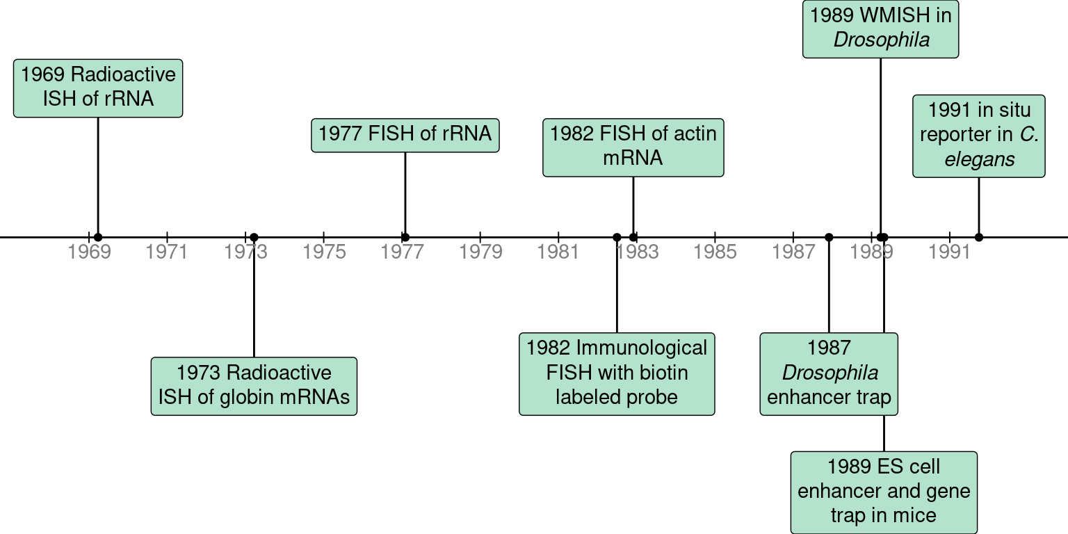
Figure 2.1: Timeline of prequel techniques.

2.1 Enhancer and gene traps

Long before the advent of reference genomes for common model organisms, the quest to characterize genes based on expression pattern in space had already begun. The earliest high-throughput efforts to identify and characterize such genes were enhancer traps. To the best of our knowledge, the first use of a reporter to visualize gene expression in space was reported in 1983. It used lacZ fused to sequences upstream to the hsp70 gene encoding a heat shock protein in Drosophila melanogaster and inserted into the genome with P element to characterize the puffs formed in polytene chromosomes and the tissue distribution of hsp70 in response to heat shock (Lis, Simon, and Sutton 1983).

The first enhancer trap screen in Drosophila melanogaster was published in 1987 (O’Kane and Gehring 1987). The P element is a transposable element found in Drosophila. In an enhancer trap vector, a reporter gene, such as lacZ, here with the polyadenylation site of the hsp70 gene, and a marker gene with its own promoter that can be used to identify individuals and their offspring with the vector integrated into the germline, such as rosy which can be used in Drosophila to identify the individuals with eye color, are flanked by the 5’ and 3’ ends of the P element necessary for transposition (Figure 2.2). The vector is injected into Drosophila embryos before the formation of pole cells (Spradling and Rubin 1982). As a transposon, the construct is randomly inserted into the genome, and since the P element promoter is so weak that an enhancer is required for the promoter to drive transcription of the reporter gene, the location of the reporter gene expression marks where the enhancer is active. As the transposon is inserted into different locations of the genome in different individuals, each individual that has the vector integrated into the germline forms a transformant line. In Drosophila, in many cases, expression patterns of \(\beta\)-galactosidase do reflect expression pattern of a nearby gene (Bellen et al. 1989; Wilson et al. 1989).

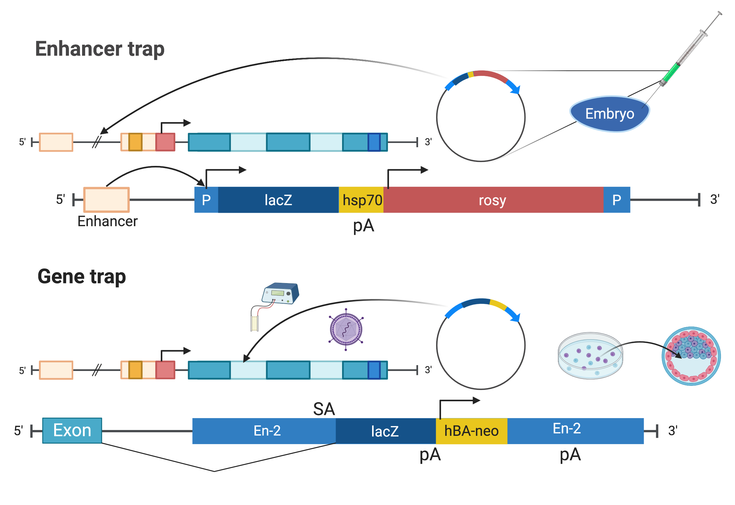
Figure 2.2: Illustrations of enhancer trap as described in (O’Kane and Gehring 1987) and gene trap as described in (Gossler et al. 1989) (Created with BioRender.com).

Since then, different vectors have been developed for better efficiency and flexibility (Stanford, Cohn, and Cordes 2001), and enhancer traps have been applied at increasing scale. The 1987 study recovered 39 lines (O’Kane and Gehring 1987), possibly characterizing 39 genes, but already in 1989, over 3000 lines were possible in one study (Bier et al. 1989). Enhancer trapping was also adapted to other species, such as mouse (Gossler et al. 1989; Allen et al. 1988) and Arabidopsis thaliana (Sundaresan et al. 1995).

Enhancer traps were not intended to be mutagenic (O’Kane and Gehring 1987), nor is it highly mutagenic (Stanford, Cohn, and Cordes 2001). Gene trap and promoter traps were introduced to not only screen for genes with restricted expression patterns, but also to enable functional analysis of the gene from homozygote mutant phenotypes (Friedrich and Soriano 1991). Like the typical enhancer trap vector, gene trap and promoter trap vectors contain a reporter gene, such as lacZ (\(\beta\)-gal), to visualize gene expression, and sometimes also a marker to screen for integration, such as the neomycin resistance gene (neo). Though often, lacZ itself, or in a fusion with neo (\(\beta\)-geo), was also used as the marker when screening mouse embryonic stem (ES) cells (Figure 2.2).

Unlike the enhancer trap vector, gene trap and promoter trap vectors do not have a promoter for the reporter, though the marker, if present, can have its own promoter. In a promoter trap, the construct needs to be inserted in frame and in the correct orientation into an exon of a gene to be expressed, making it very inefficient (Friedrich and Soriano 1991; Stanford, Cohn, and Cordes 2001).

In contrast, in gene traps, a splice acceptance site is added to the 5’ end of the reporter, so the construct can be expressed when inserted into an intron at the right orientation; this is over 50 times more efficient than a promoter trap because introns tend to be much longer than exons and the construct does not have to be in frame to an exon (Friedrich and Soriano 1991; Stanford, Cohn, and Cordes 2001). Gene traps and promoter traps are mutagenic as the reporter has a stop codon, thus truncating the endogenous protein.

While enhancer traps are more commonly used in Drosophila, gene traps are more commonly used in mice. In mice, in 1988, the enhancer trap vector was initially introduced by injection into the male pronucleus in the fertilized egg (Allen et al. 1988). The throughput of the screen is increased by inserting the construct into genomes of ES cells by electroporation or retroviral infection (Stanford, Cohn, and Cordes 2001), screening for ES cells expressing lacZ or the marker, injecting these ES cells into blastocysts to generate chimeric mice to characterize gene expression patterns; chimera are especially useful for characterizing dominant and lethal mutations (Friedrich and Soriano 1991; Gossler et al. 1989).

The first gene trap screen in mouse ES cells was reported in 1989 (Gossler et al. 1989), recovering 14 lines. Again, variants of the vector emerged and gene trap screens increased in scale. In 1995, nearly 300 mouse gene trap lines were recovered from one study (Wurst et al. 1995). Later, smaller gene trap studies specific to particular types of genes made possible by additional steps to screen ES cell colonies were performed, such as genes encoding membrane and secreted proteins (Skarnes et al. 1995), genes responding to retinoic acid (Forrester et al. 1996), and genes expressed in hematopoitic and endothelial lineages (Stanford et al. 1998). In 2001, gene trapping was used to examine not only expression pattern of genes in cell bodies of neurons in the mouse brain, but also axon guidance (Leighton et al. 2001). By 2001, a number of gene trap consortia have been established as resources of gene trap vectors and transformant mouse ES cell lines, hoping to create at least one line for each gene in the mouse genome (Stanford, Cohn, and Cordes 2001).

In the 1980s and 1990s, with increasing throughput of Sanger sequencing and the advent of shotgun sequencing, the amount of sequencing data in GenBank exploded (Giani et al. 2020). With 5’ or 3’ rapid amplification of cDNA ends (RACE) PCR, the fusion transcript of the reporter and an endogenous gene could be cloned (Frohman, Dush, and Martin 1988), sequenced, and potentially aligned to the existing sequences to identify the gene of interest (Stanford et al. 1998). However, the golden age of gene trapping was soon to pass, with the rise of ISH atlases in the late 1990s and the advent of reference genomes of Drosophila melanogaster (Myers 2000), mouse (Waterston et al. 2002), and human (Lander et al. 2001; Venter et al. 2001) in the early 2000s that would make it easier to design ISH probes from the reference genome to target annotated genes, as is done today. Nevertheless, enhancer and gene traps were not rendered obsolete by these developments. They have been used in plants and zebrafish through the 2000s and 2010s, as resources of gene expression patterns (Johnson et al. 2005; Nakayama et al. 2005; Pérez-Martín et al. 2017; Hiwatashi et al. 2001; Kawakami et al. 2010; Marquart et al. 2015) (Figure 2.3).

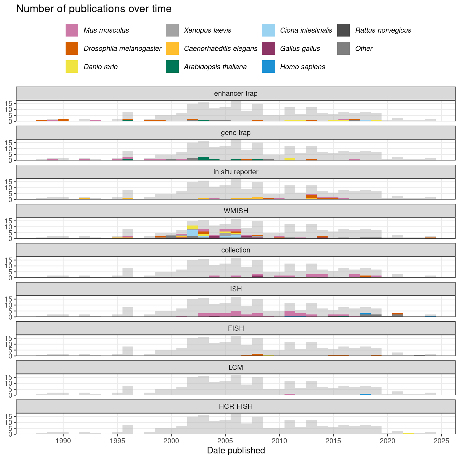
Figure 2.3: Number of publications over time in the prequel era, broken down by technique and colored by species. The gray histogram in the background is the histogram for all prequel publications over time. The bin width of this histogram is 365 days. Here WMISH and ISH exclude fluorescent ISH (FISH).

2.2 In situ reporter

In enhancer, gene, or promoter trap screens, the reporter is randomly inserted into the genome, not targeting predetermined genes. In contrast, in what we call in situ reporter screens, the reporter is fused to predefined regulatory sequences of a gene of interest, with the hope that expression pattern of the reporter would recapitulate that of the gene of interest. Chronologically, this is the second type of high throughput method to profile gene expression patterns (Figure 2.3).

A precursor to this type of method was used in 1991, where random genomic fragments were fused to a lacZ reporter lacking a transcription start signal and injected as plasmids, screening for fragments driving lacZ expression and characterizing the expression patterns in C. elegans (Hope 1991). To the best of our knowledge, the first time in situ reporter with predefined regulatory sequences was used to screen for gene expression patterns in a multicellular organism, was in 1995, in C. elegans (Lynch, Briggs, and Hope 1995). At that time, the C. elegans genome sequencing project was already in progress (Lynch, Briggs, and Hope 1995; Sulston et al. 1992), and the genome sequence was declared “essentially complete” in 1998 (Consortium 1998). Computationally predicted upstream regulatory sequences of 35 putative genes were fused to a promoterless lacZ as a reporter, cloned into plasmid vectors, and microinjected into C. elegans gonads to create transformed lines then stained with X-gal (Lynch, Briggs, and Hope 1995).

A reliable in situ reporter was first reported in mice in 1997. It used a recombinant bacterial artificial chromosome (BAC) with part of the full RU49 gene in the BAC replaced by a lacZ construct and showed that the construct is heritable (X. W. Yang, Model, and Heintz 1997). In 2003, a similar strategy, replacing coding sequences of genes in BACs with EGFP reporter gene, was used to create a mouse brain gene expression atlas GENSAT with BAC transgenic mouse lines (Gong et al. 2003). The GENSAT lines were used again in 2009 to create a gene expression atlas for retina (Siegert et al. 2009). Again, GENSAT benefited from the reference genome, which greatly helped with identifying BACs that include sequences flanking a gene that may contain regulatory elements that make the reporter better recapitulate expression pattern of the endogenous gene (Gong et al. 2003).

Through the 2000s and 2010s, in situ reporters have been used as a targeted alternative to enhancer and gene trap screens informed by the reference genomes. To address limitations of gene traps, such as inability to precisely define the allele and favoring genes expressed in ES cells when screening for transformant colonies, high-throughput mouse knock out resources with knock out alleles computationally designed according to a reference genome and annotations have been established (Skarnes et al. 2011; “A Mouse for All Reasons” 2007). As these alleles contain a lacZ reporter, these resources have been used to characterize gene expression in over 40 tissues in mutant mice with lacZ staining (White et al. 2013; West et al. 2015; Tuck et al. 2015). However, for some tissues, only low resolution whole mount staining was performed. Similarly, in both mouse (Visel et al. 2013) and Drosophila (Jenett et al. 2012; Kvon et al. 2014), transgenic lines with genomic fragments containing putative enhancers driving expression of reporter genes were established as alternatives to enhancer traps. The enhancer candidates can be selected from sequence homology and ChIP-seq predictions (Visel et al. 2013), or from tiles of sequences flanking genes thought to have restricted expression patterns or within introns of such genes (Jenett et al. 2012).

In situ reporter atlases exceeded the scale of enhancer and gene trap screens. The largest such atlas in C. elegans, WormAtlas, profiled 1886 genes (Hunt-Newbury et al. 2007); we are unaware of enhancer and gene trap screens in C. elegans because C. elegans genome sequencing was already underway by 1992 (Sulston et al. 1992), making in situ reporter screening feasible before it was so in mice and Drosophila. The largest such study in Drosophila profiled 7705 enhancer candidates (Kvon et al. 2014), which far exceeded the 3768 enhancer trap lines in 1989 (Bier et al. 1989). In situ reporters were used in mice to profile up to 536 genes(Siegert et al. 2009) and 329 enhancer candidates (Visel et al. 2013), while the large scale gene trap screen in 1995 only reached 279 lines (Wurst et al. 1995) and later mouse gene trap screens did not typically exceed 100 lines. However, where comparable, in situ reporter atlases never reached the scale of (WM)ISH atlases, perhaps because of the large number of transgenic lines required. Allen Brain Atlas (ABA) profiled over 20,000 genes in the mouse brain, and as of April 2021, the Berkeley Drosophila Genome Project (BDGP) WMISH atlas already has 8533 genes. However, in situ reporters might still be a good way to profile enhancer usage in space.

2.3 ISH and WMISH atlases

In situ hybridization was first used in 1969 to visualize ribosomal RNA (rRNA) (Gall et al. 1969) and ribosomal DNA (rDNA) (John, Birnstiel, and Jones 1969) in Xenopus laevis oocytes with probes labeled with radioisotope ³H (Figure 2.1). To the best of our knowledge, the earliest use of ISH to visualize what was thought to be a specific transcript was done in 1973, to visualize globin mRNAs in various cultured erythroid and non-erythoid cell types by hybridization of radiolabeled cDNA to the mRNA (Harrison et al. 1973). As radioactive ISH requires long exposure time (several weeks), has low spatial resolution and high background, and requires handling hazardous radioactive material, alternatives emerged in the mid 1970s and early 1980s. Among the alternatives were variants of FISH and labeled probes detected by primary and enzyme or fluorophore labeled secondary antibodies (Huber, Voithenberg, and Kaigala 2018; Langer-Safer, Levine, and Ward 1982); the latter, immunological method is commonly used in ISH and WMISH atlases. To the best of our knowledge, the first report of using immunological fluorescent and peroxidase ISH to visualize expression of a specific gene was published in 1982, the same year such technique was published (Langer-Safer, Levine, and Ward 1982), visualizing actin transcripts in chicken muscle tissue culture; the authors reported puncta of cytoplasmic fluorescence which might be clumps of mRNAs or artefact, but could possibly be individual transcripts (Singer and Ward 1982).

Non-radioactive ISH not only has shorter exposure time and higher resolution than radioactive ISH, but also made WMISH possible. WMISH was first reported in Drosophila embryos in 1989 (Tautz and Pfeifle 1989), and was adapted to other model organisms such as mice, Xenopus laevis, and Paracentrotus lividus (purple sea urchin) in the early 1990s (Rosen and Beddington 1993). Advantages of WMISH compared to section ISH is preservation of 3D structure of the tissue, ease of interpretation in blastoderm stage embryos, and ease of performing ISH on larger number of embryos (Rosen and Beddington 1993; Tautz and Pfeifle 1989).

Just like genome sequencing in multi-cellular organisms and in situ reporter screens, WMISH atlases got a head start in C. elegans. The first WMISH screen with higher throughput than typically used on select marker genes was reported in 1994, of 21 genes in C. elegans (Seydoux and Fire 1994). Early (WM)ISH atlases in the late 1990s typically made probes from cDNA clones from poly-A selected RNAs in tissue or developmental stage of interest without pre-selecting genes to stain for (Tomancak et al. 2002; Stapleton 2002; Gawantka et al. 1998; Bettenhausen and Gossler 1995). Some early atlases were intended to be improvements to enhancer and gene trapping and in situ reporter screens, as a simpler and more direct alternative (Bettenhausen and Gossler 1995) or as a way that can better capture endogenous and dynamic spatial distribution of transcripts (Gawantka et al. 1998). Since 1998, (WM)ISH has been automated, enabling staining for thousands of probes (Gawantka et al. 1998; Carson, Thaller, and Eichele 2002).

The genes from which the clones come from were often unknown, so early (WM)ISH atlases referred to the entities stained for as “clones” (Figure 2.4), though the genes, homology, and putative functions of the genes can be identified by aligning sequences of the cDNA clones to existing sequences in databases (Bettenhausen and Gossler 1995; Gawantka et al. 1998; Kopczynski et al. 1998). However, again, the first WMISH screen with probes made from cloning PCR amplified pre-defined genomic sequences was performed in C. elegans in 1995 (Birchall, Fishpool, and Albertson 1995). By the turn of the century, the entities stained for were sometimes referred to as “clusters”, especially in the GHOST atlas for Ciona intestinalis (Satou et al. 2001) (Figure 2.4); the sequences of the probes were clustered by alignment and these probes might have come from the same gene.

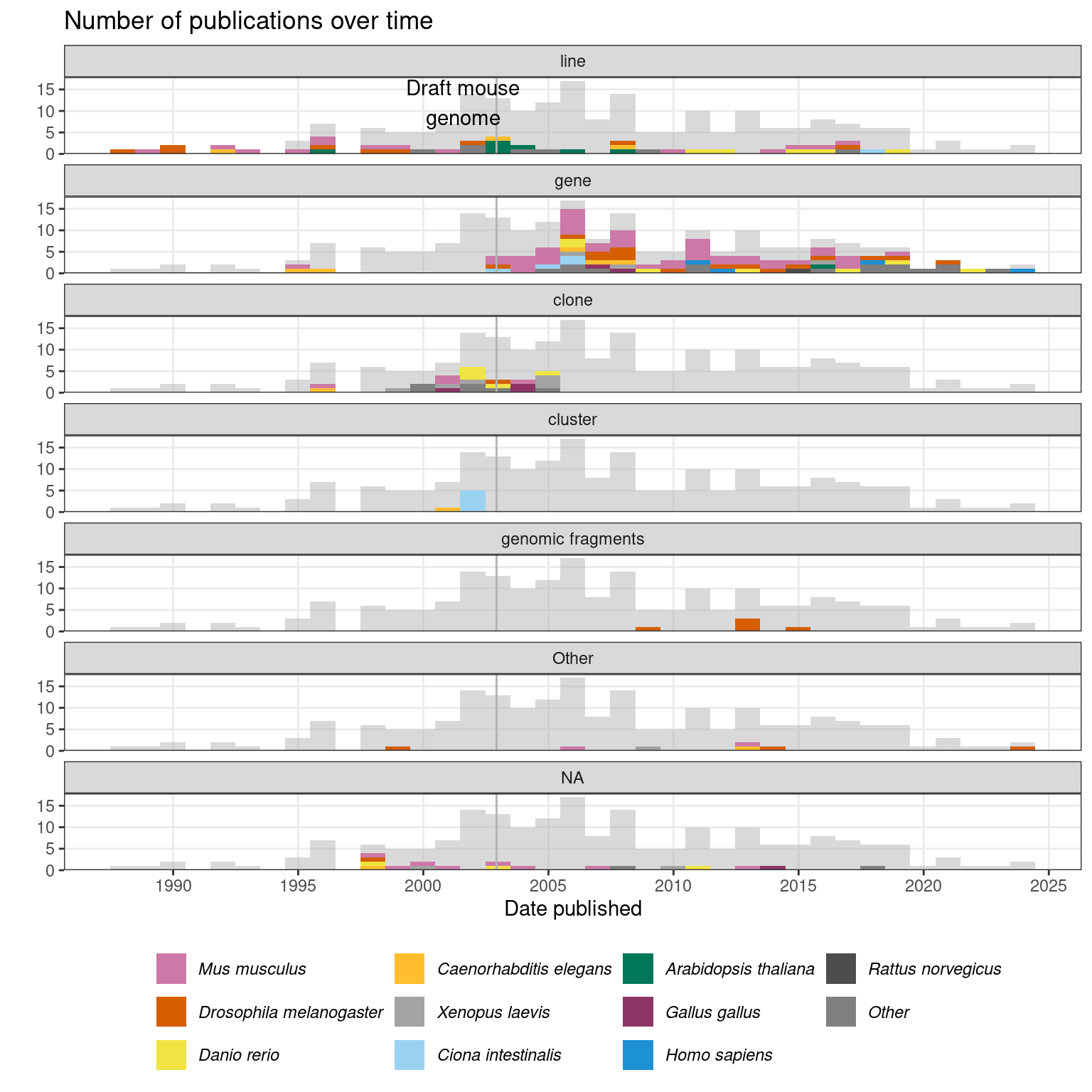
Figure 2.4: Number of prequel publications over time, broken down by what the entities stained for were called and colored by species. Bin width is 365 days. Vertical line marks the date when the draft mouse reference genome was published (Waterston et al. 2002), as context of transition from “clone” and “line” to “gene”.

The rise of (WM)ISH atlases started before the completion of genome projects in humans and common model organisms, although their later growth was transformed by the reference genome. In the 2000s, with the availability of sequenced cDNA collections covering increasing proportion of predicted genes and the consequent rise of transcriptome-wide microarray (Stapleton 2002; Carter 2003), genes to be stained for in (WM)ISH atlases could be pre-screened based on microarray data of the tissue of interest, with probes made from cDNA clones readily available from such collections (Yoshikawa et al. 2006; E. S. Lein 2004). In addition, probes could be computationally designed based on reference genome sequences (E. S. Lein et al. 2007). Perhaps because of these developments, since the turn of the century, entities stained for have been predominantly referred to as “genes” (Figure 2.4). Notably, while radioactive ISH has been mostly replaced by non-radioactive ISH by the 2000s, there is a mouse hippocampus ISH atlas published in 2004 that used radioactive ISH to profile all of its 104 genes (E. S. Lein 2004).

Also with the rise of cDNA microarray in the late 1990s and early 2000s, some (WM)ISH atlases were made as an improvement to microarray with bulk tissue to profile the transcriptome, not only at cellular resolution, but also preserving spatial and sometimes temporal context (E. S. Lein et al. 2007; Bell, Yatskievych, and Antin 2004), analogous to how scRNA-seq and various later forms of spatial transcriptomics were developed in response to bulk RNA-seq.

Since the 2000s, (WM)ISH atlases have been made for specific types of genes and a number of mouse tissues. In 2004, locked nucleic acid (LNA) modified oligonucleotide probes were introduced, greatly improving sensitivity of miRNA northern blot (Valoczi 2004) and made (WM)ISH atlases for miRNAs possible. The first miRNA WMISH atlas was published in 2005, which profiled 115 miRNAs in zebrafish embryos (Wienholds 2005). Since then, miRNA atlases were created for mice (Karali et al. 2010; Diez-Roux et al. 2011; Kloosterman et al. 2006), Drosophila (Aboobaker et al. 2005), chicken (Darnell et al. 2006), and Xenopus laevis (Ahmed et al. 2015).

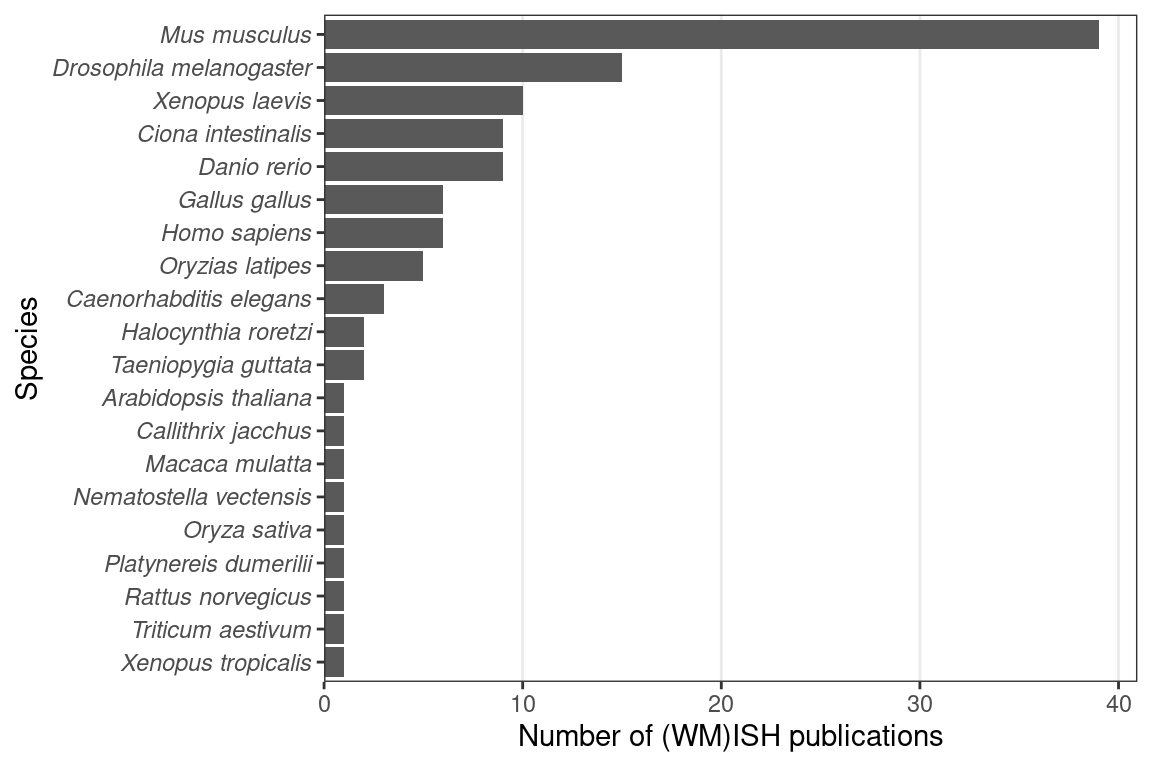
Figure 2.5: Number of (WM)ISH publications per species.

While (WM)ISH atlases are available for several species, the mouse is by far the favored model organism (Figure 2.5). A timeline of the first (WM)ISH atlas for each of the species and some notable atlases are shown in Figure 2.6. Especially for mice, atlases for other specific types of genes were published in the late 2000s and the 2010s, such as genes coding for RNA binding proteins (McKee et al. 2005), fibroblast growth factors and their receptors (Yaylaoglu et al. 2005), proteins with catalytic activities (Cankaya et al. 2007), transcription factors and cofactors (Yokoyama et al. 2009), metabolic enzymes and soluble carriers (Geffers et al. 2012), cholesterol biosynthetic enzymes (Şişecioğlu et al. 2015), and ion channels (in rats) (Shcherbatyy et al. 2015). Among the mouse atlases, while the brain gets disproportionately strong interests, with the influential ABA (E. S. Lein et al. 2007) and GenePaint (Carson, Thaller, and Eichele 2002), ISH atlases exist for the eye (Thut et al. 2001; Blackshaw et al. 2004), genitourinary tract (GenitoUrinary Development Molecular Anatomy Project (GUDMAP)) (Harding et al. 2011), and lung (LungMAP) (Ardini-Poleske et al. 2017) (Figure 2.6, Figure 2.7).

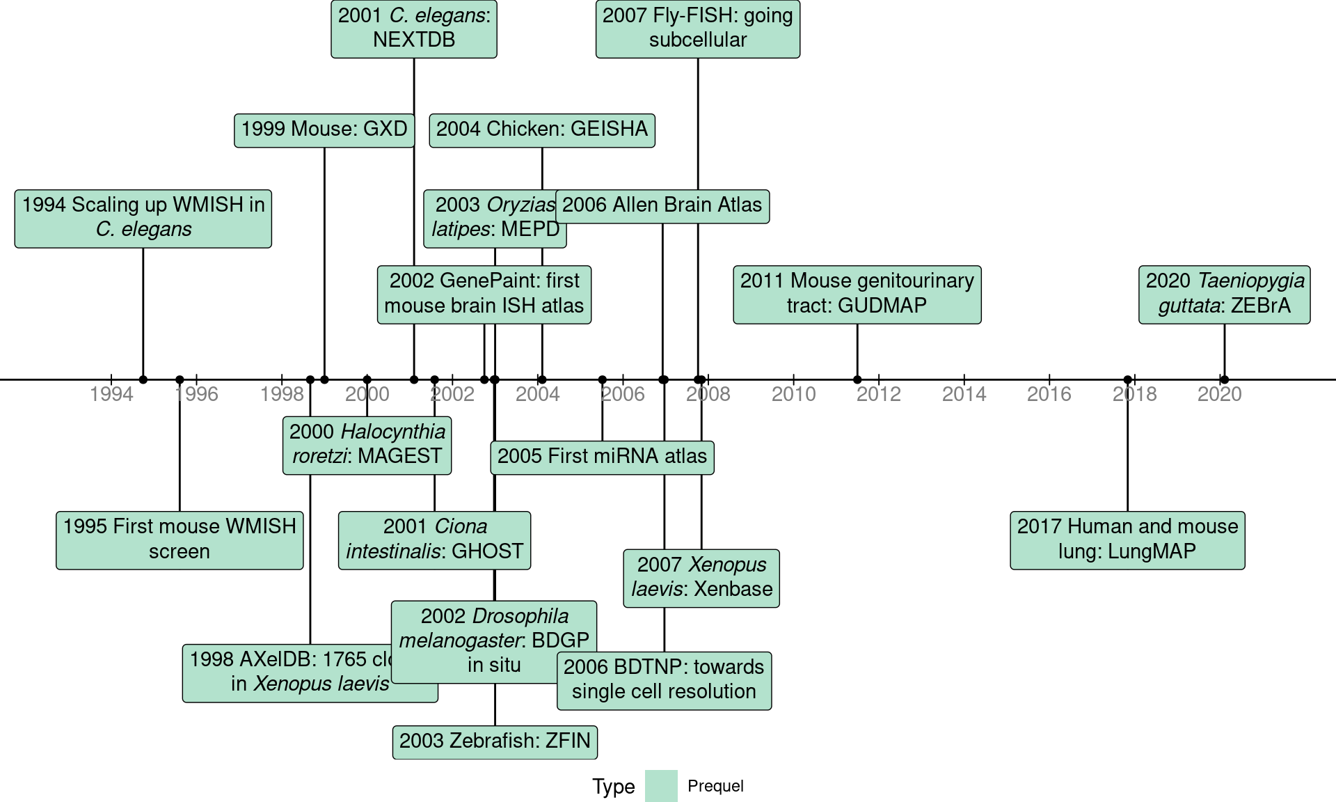
Figure 2.6: Timeline of the first (WM)ISH databases for each species for which such databases are available, as well as some notable databases.

While the vast majority of (WM)ISH atlases used bright field imaging, a few used FISH (Figure 2.3), for advantages conferred by FISH discussed below. A notable FISH atlas is the Berkeley Drosophila Transcription Network Project (BDTNP) from 2006 to 2008, which profiled expression patterns of 95 genes in the Drosophila embryo across 6 developmental stages up to the beginning of gastrulation (Fowlkes et al. 2008; Hendriks et al. 2006). Two genes are imaged in each embryo, and the images of 1822 embryos were registered across both space and time to construct 3D virtual embryos on which patterns of different genes can be quantitatively compared (Fowlkes et al. 2008); the 3D imaging and penetration into the opaque yolk is made possible by two photon microscopy, in which only the fluorophores in the region of focus are excited (Hendriks et al. 2006). Another notable FISH atlas is Fly-FISH from 2007, which profiled subcellular localization of transcripts of 3370 genes in Drosophila embryos (Lécuyer et al. 2007). While subcellular localization of transcripts can sometimes be discerned in bright field WMISH (Tomancak et al. 2002), Fly-FISH shows higher subcellular resolution thanks to a FISH protocol using tyramide signal amplification. To our best knowledge, this is the first transcriptomic atlas of a multi-cellular organism to profile subcellular transcript localization. While more recent smFISH based methods record subcellular information, such information is typically not used in downstream analyses.

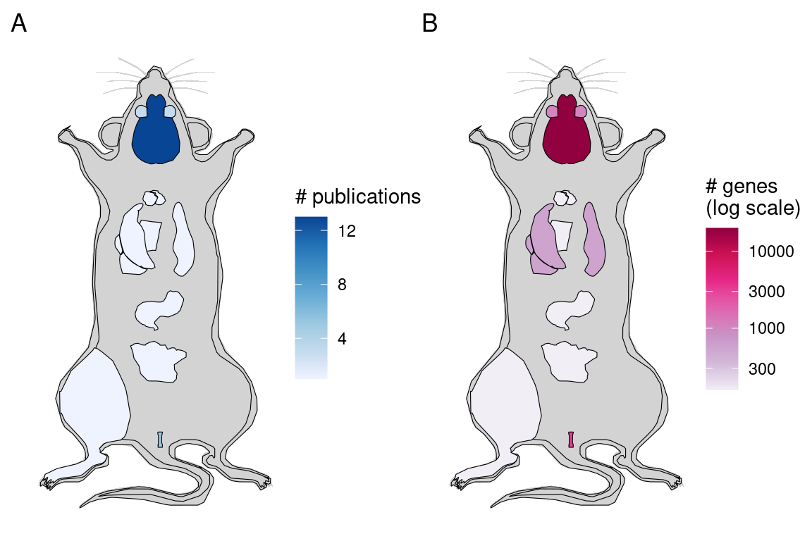
Figure 2.7: A) Number of mouse publications per organ for (WM)ISH atlases (including FISH). B) Maximum number of genes in atlases for each organ, as of publication of the paper about the atlases. The color is in log scale to improve dynamic range.

WMISH was the most commonly used technique in the prequel era, followed by ISH (Figure 2.8). In summary, advances of non-radioactive ISH and WMISH from radioactive ISH, limitations of enhancer and gene trap and in situ reporter screens, cDNA collections that cover most of predicted genes, limitations of bulk microarray, reference genomes that allow for computational probe design, and ISH robots may have been responsible for the rise of (WM)ISH atlases. Another important factor may be the rise of digital photography and the internet in the 1990s, as developing thousands of analogue photos is an arduous task. Moreover, online digital atlases have been much more accessible to the wider community. Assuming that the number of publications in a field reflects interest in that field during a period of time, and if our collection is representative of the actual body of literature, then the golden age of the prequel era was the 2000s and WMISH was responsible for that peak, while section ISH and “collection”, i.e. databases of gene expression patterns curated from publications and some (WM)ISH atlases, account for much of the interest after 2010 (Figure 2.3). The websites of many of the older (WM)ISH atlases are no longer accessible. However, some of the atlases from that period of time still live on in extant curated databases, which will be discussed in the next section.

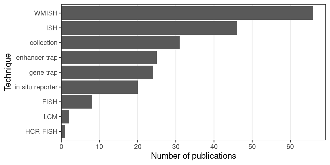
Figure 2.8: Number of prequel publications per technique.

The golden age declined before the rise of current era spatial transcriptomics, which started around 2014 4.2. What contributed to the decline of the golden age? Perhaps with proliferation of such atlases, curated databases exceeding 10,000 genes, and especially with over 20,000 genes in ABA mapped to a high quality 3D mouse brain model, there are already enough gene expression pattern resources for the most commonly studied genes, tissues (especially the brain), and developmental stages in the most common model organisms, thus making new atlases in those systems unnecessary. Moreover, in the last decade, the under-utilization of gene expression atlases (Boer et al. 2009) may have reduced motivation to build new atlases. Or perhaps, more importantly, inherent limitations of non-multiplexed (WM)ISH contributed to the decline in interest in such methods. In these atlases, typically only one gene is stained for in each individual embryo or tissue section. Gene expression patterns of different genes can only be meaningfully compared and classified in tissues with a stereotypical structure, such as wild type embryos and the brain, but not tumors and pathological tissues, even though there is intense interest in spatial transcriptomics in tumors as evidenced by the LCM and ST literature 6.3. A large number of embryos or sections are required for such atlases, thus increasing cost and making human atlases extremely difficult and costly, if ethical at all. Furthermore, since the chromogenic reaction in bright field ISH can be prolonged to increase staining intensity, the patterns are not quantitative and consequently, analyses of such patterns typically involve binarization and quantitative expression levels of genes cannot be compared. Even with a stereotypical structure, image registration can be challenging because of biological differences between individuals (Fowlkes et al. 2008).

2.4 Databases of the prequel era

Many of the (WM)ISH atlases discussed above, such as BDGP (Tomancak et al. 2002), Gallus In Situ Hybridization Atlas (GEISHA) (Bell, Yatskievych, and Antin 2004), ABA (E. S. Lein et al. 2007), BDTNP (Fowlkes et al. 2008), GUDMAP (Harding et al. 2011), and LungMAP (Ardini-Poleske et al. 2017) are stored in databases that can be queried online, typically by gene symbol or by controlled anatomical or developmental vocabulary (i.e. ontology, reviewed in depth in (Clarkson 2016)). There are additional gene expression databases for images curated from publications, some containing non-spatial data as well and some specifically for spatial data.

The rise of the curated databases started in the 1990s. Already in 1992, the challenges of managing the increasing amount of gene expression data in developmental biology emerged and a spatiotemporal database of mouse gene expression that would later become the Edinburgh Mouse Atlas of Gene Expression (EMAGE) was discussed (Baldock et al. 1992). In 1994, Jackson Laboratory proposed the Gene Expression Database (GXD) (Ringwald et al. 1994), in collaboration with EMAGE to build the most comprehensive mouse gene expression database. In 1997, work was already in progress to produce (WM)ISH atlases and construct the database infrastructure for mouse (Ringwald et al. 1997) (GXD and EMAGE), Drosophila melanogaster (Janning 1997), C. elegans (Martinelli, Brown, and Durbin 1997), and zebrafish (Westerfield et al. 1997). Curated databases of mice (GXD and EMAGE), zebrafish (Zebrafish Information Network (ZFIN) (Howe et al. 2017)), and Xenopus laevis (Xenbase (Bowes et al. 2009)) were released in the 2000s, within a tide of (WM)ISH atlases for new species (Figure 2.6). Some of these databases are regularly updated and the updates are responsible for many of the “collection” publications after 2010 (Figure 2.3, Figure 2.8); our historical literature collection has not only the original publications for the databases, but also publications for later updates that involve new spatial gene expression images. Examples of other extant curated databases: for Drosophila melanogaster FlyExpress (Kumar et al. 2017), for Xenopus laevis XenMARK (Gilchrist et al. 2009), and for ascidians Ascidian Network for In Situ Expression and Embryological Data (ANISEED) (Tassy et al. 2010). Databases, curated or not, are available for several species; mice, Drosophila, and zebrafish have the most extant databases (Figure 2.9).

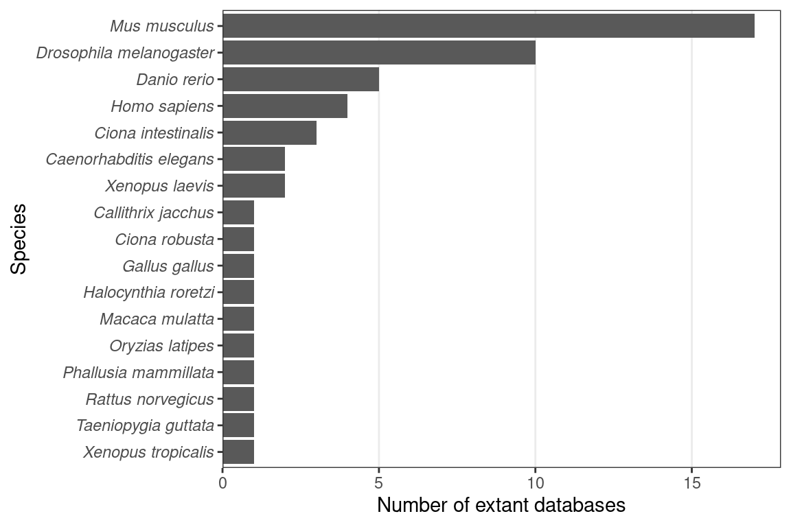
Figure 2.9: Number of extant spatial gene expression databases per species.

Data can be exchanged between databases. For example, among mouse databases GenePaint (Carson, Thaller, and Eichele 2002) and EMAGE now contain data from Eurexpress (Diez-Roux et al. 2011; Boer et al. 2009), and EMAGE uses data from GXD for the 3D gene expression models (Ringwald et al. 1999). ANISEED contains data from WMISH atlases GHOST for Ciona intestinalis (Satou et al. 2001) and MAboya Gene Expression patterns and Sequence Tags (MAGEST) for Halocynthia roretzi (Kawashima 2000). FlyExpress contains data from Drosophila atlases such as BDGP and Fly-FISH. Data in databases that ceased to operate may still be available in extant databases. For instance, AXelDb WMISH atlas and database for Xenopus laevis (Gawantka et al. 1998) has been subsumed in Xenbase while AXelDb’s own website has long been defunct. Likewise, as of April 2021, the MAGEST website is defunct but the data lives on in ANISEED.

Some of the databases go beyond collecting data from other databases. Databases such as EMAGE, ANISEED, and ABA registered multiple 2D section images to map gene expression patterns onto 3D anatomical models for better comparison between different genes. FlyExpress also standardized the images from the atlases and enables search for coexpressed genes by expression pattern (Kumar et al. 2017). There have also been efforts to integrate databases from multiple model organisms. In 2007, COMPARE (Salgado et al. 2008) and 4DXpress (Haudry et al. 2007) were developed to make gene expression patterns and developmental stages in zebrafish, mouse, and Drosophila (also medaka in 4DXpress) comparable. While COMPARE and 4DXpress are no longer available, interest in integrating the databases continues, so in 2016, the Alliance of Genome Resource was founded, producing a unified user interface to genome and gene expression databases for Saccharomyces cerevisiae, C. elegans, Drosophila melanogaster, mouse, rat, and zebrafish (Agapite et al. 2020), although spatial patterns are not its focus.

2.5 Geography of the prequel era

Where were prequel era research conducted? Our database includes affiliation of the first author as of publication for all papers, and the affiliations have been geocoded to plot on maps. Around the world, most of prequel studies were performed in coastal US and Western Europe, but a some studies were performed in Asia and Oceania, but especially Japan (Figure 2.10). Not all of the top contributing institutions are readily recognizable “elite” institutions. Institutions include BDGP from UC Berkeley, ZFIN from University of Oregon (UO), ABA from Allen Brain Institute (Allen), GEISHA from University of Arizona (UofA), GXD from Jackson Laboratory (JAX), EMAGE from Western General Hospital (WGH), MEPD (for Oryzias latipes) from European Molecular Biology Laboratory (EMBL), and GHOST from Kyoto University (Kyodai), and mouse gene trap lines from Mount Sinai.

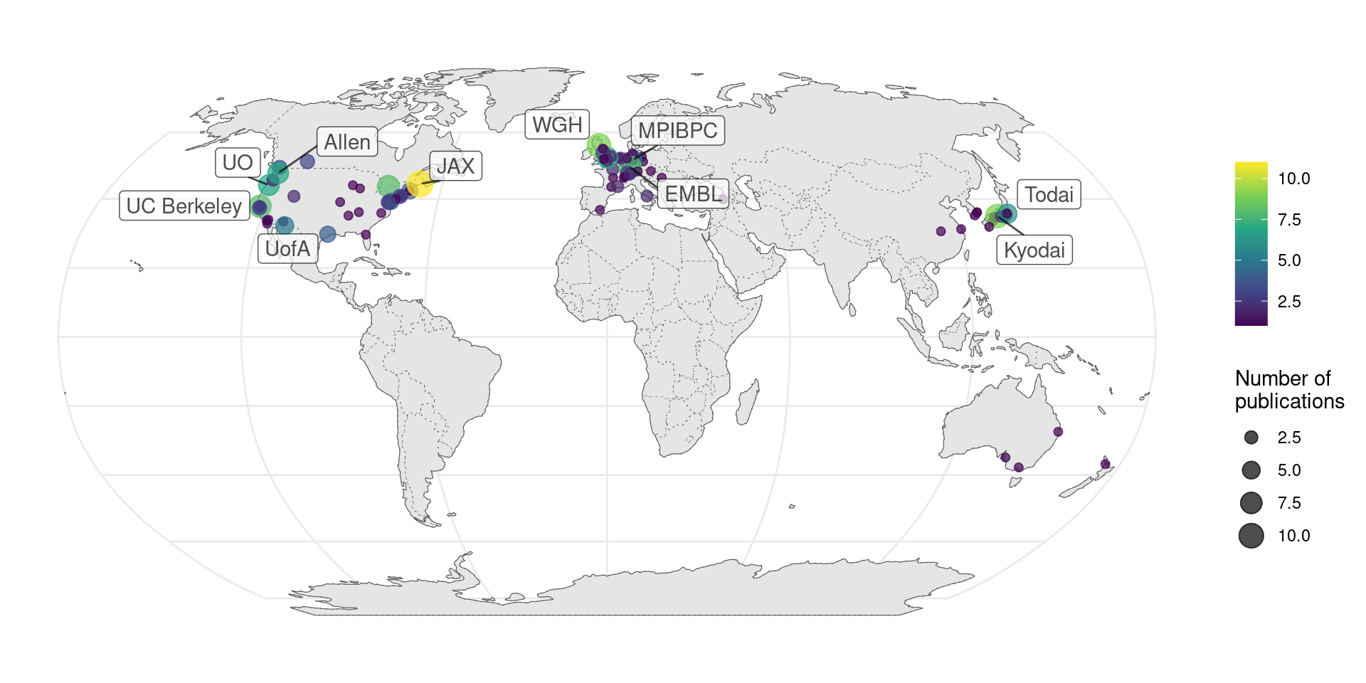
Figure 2.10: Number of prequel publications per city around the world, with top contributing institutions labeled.

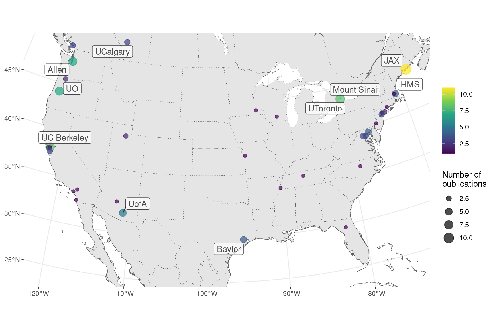
Figure 2.11: Number of prequel publications in the US and Canada, with top contributing institutions labeled.

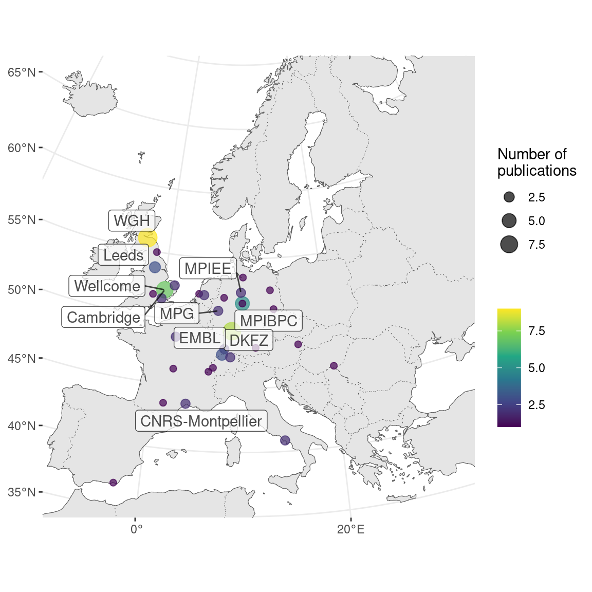
Figure 2.12: Number of prequel publications in western Europe, with top contributing institutions labeled.

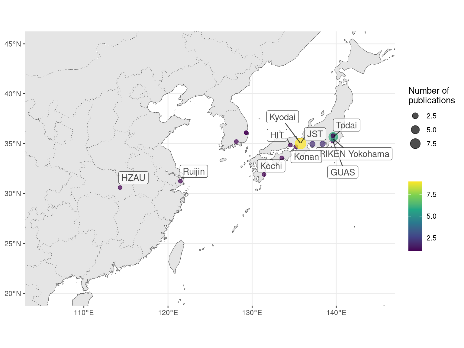
Figure 2.13: Number of prequel publications in northeast Asia, with top contributing institutions labeled.

This can be better visualized by breaking the map down by species. Here we see locations of some model organism consortia, and that GHOST is a result of collaboration of multiple Japanese institutions (Figure 2.14).

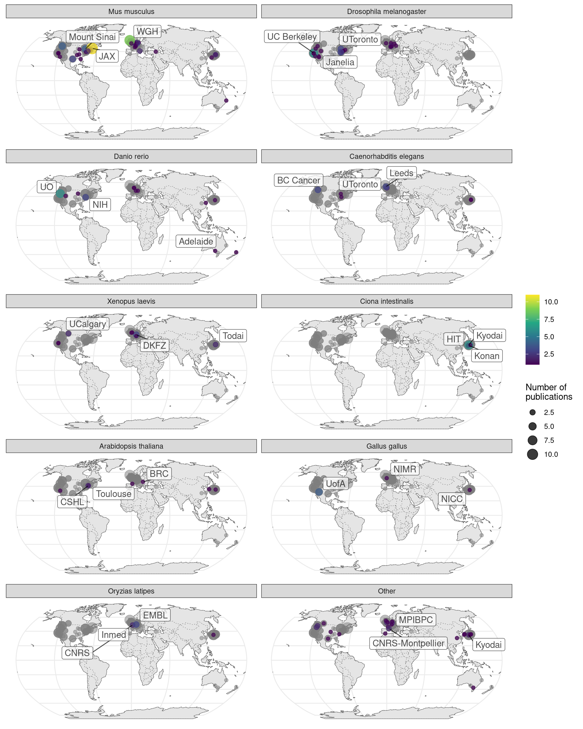
Figure 2.14: Number of prequel publications per city broken down by species. Gray points are the overall number as a reference of contributions from each city and region.

That some institutions have disproportional contribution of one technique can also be shown. Here it’s clear that prequel techniques are used by many different institutions (Figure 2.15). In contrast, as will be shown in Chapter 4, most current era techniques never spread beyond their institutions of origin. The LCM study comes from Allen Brain Institute’s atlases for Allen’s mouse sleep deprivation atlas (Thompson et al. 2010) and human glioblastoma atlas (Puchalski et al. 2018); although LCM is a current era technique, those two studies are in the prequel sheet because they also have ISH atlases.

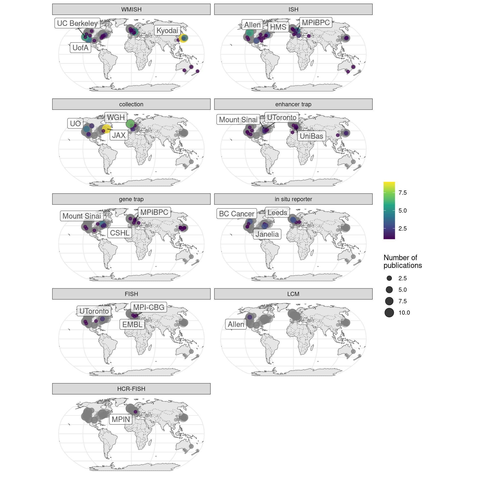
Figure 2.15: Number of prequel publications per city broken down by technique. Gray points are the overall number as a reference of contributions from each city and region.