Skip to contents

Introduction

In a more introductory vignette, we performed basic non-spatial analyses on a mouse olfactory bulb Visium dataset from the 10X website. In this vignette, we perform spatial analyses in histological space as well as in gene expression space.

Here we load the packages used in this vignette:

# Specify Python version to use gget
PY_PATH <- system("which python", intern = TRUE)
use_python(PY_PATH)
py_config()
#> python:         /Users/runner/hostedtoolcache/Python/3.10.13/x64/bin/python
#> libpython:      /Users/runner/hostedtoolcache/Python/3.10.13/x64/lib/libpython3.10.dylib
#> pythonhome:     /Users/runner/hostedtoolcache/Python/3.10.13/x64:/Users/runner/hostedtoolcache/Python/3.10.13/x64
#> version:        3.10.13 (main, Aug 28 2023, 08:29:32) [Clang 13.0.0 (clang-1300.0.29.30)]
#> numpy:          /Users/runner/hostedtoolcache/Python/3.10.13/x64/lib/python3.10/site-packages/numpy
#> numpy_version:  1.26.2
#> 
#> NOTE: Python version was forced by use_python() function
gget <- import("gget")

Here we download the data from the 10X website. This is the unfiltered gene count matrix:

if (!file.exists("visium_ob.tar.gz"))
    download.file("https://cf.10xgenomics.com/samples/spatial-exp/2.0.0/Visium_Mouse_Olfactory_Bulb/Visium_Mouse_Olfactory_Bulb_raw_feature_bc_matrix.tar.gz", 
                  destfile = "visium_ob.tar.gz")

This is the spatial information:

if (!file.exists("visium_ob_spatial.tar.gz"))
    download.file("https://cf.10xgenomics.com/samples/spatial-exp/2.0.0/Visium_Mouse_Olfactory_Bulb/Visium_Mouse_Olfactory_Bulb_spatial.tar.gz", 
                  destfile = "visium_ob_spatial.tar.gz")

Decompress the downloaded content:

if (!dir.exists("outs")) {
    dir.create("outs")
    system("tar -xvf visium_ob.tar.gz -C outs")
    system("tar -xvf visium_ob_spatial.tar.gz -C outs")
}

Contents of the outs directory as from Space Ranger is explained in the introductory vignette.

Here we read the data into R as an SFE object.

(sfe <- read10xVisiumSFE(samples = ".", type = "sparse", data = "raw"))
#> class: SpatialFeatureExperiment 
#> dim: 32285 4992 
#> metadata(0):
#> assays(1): counts
#> rownames(32285): ENSMUSG00000051951 ENSMUSG00000089699 ...
#>   ENSMUSG00000095019 ENSMUSG00000095041
#> rowData names(8): symbol Feature.Type ...
#>   Median.Normalized.Average.Counts_sample01
#>   Barcodes.Detected.per.Feature_sample01
#> colnames(4992): AAACAACGAATAGTTC-1 AAACAAGTATCTCCCA-1 ...
#>   TTGTTTGTATTACACG-1 TTGTTTGTGTAAATTC-1
#> colData names(4): in_tissue array_row array_col sample_id
#> reducedDimNames(0):
#> mainExpName: NULL
#> altExpNames(0):
#> spatialCoords names(2) : pxl_col_in_fullres pxl_row_in_fullres
#> imgData names(4): sample_id image_id data scaleFactor
#> 
#> unit: full_res_image_pixel
#> Geometries:
#> colGeometries: spotPoly (POLYGON) 
#> 
#> Graphs:
#> sample01:

Here we add QC metrics, already plotted in the introductory vignette.

is_mt <- str_detect(rowData(sfe)$symbol, "^mt-")
sfe <- addPerCellQCMetrics(sfe, subsets = list(mito = is_mt))

Tissue segmentation

While Space Ranger can automatically detect which spots are in tissue and the Loupe browser can be used to manually annotate which spots are in tissue, it may be interesting to get the tissue outline polygon, so we would know how much each spot overlaps with the tissue and plot the outline. The tissue boundary polygon can be manually annotated with QuPath, which saves the polygon as a GeoJSON and can be directly read into R with st_read().

Or we can segment the tissue computationally. R generally isn’t great for image processing, but there are some packages that can perform the segmentation, such as EBImage, which is based on its own in house C and C++ code, and imager, which is based on CImg.

Here we don’t have the full resolution image. We will perform tissue segmentation on the high resolution downsampled image and then scale it to make the coordinates of the tissue boundary match those of the spots. The EBImage package is used here. Compared to OpenCV, EBImage is slow on the full resolution image, but should be fine here for the downsized image.

img <- readImage("outs/spatial/tissue_hires_image.png")
display(img)

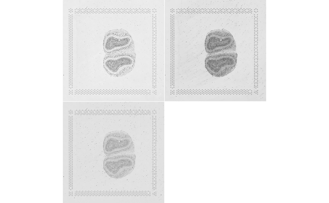
When rendered as a static webpage, the image is static, but when run interactively, this image will be shown in an interactive widget where you can zoom and pan.

Here we show the RGB channels separately
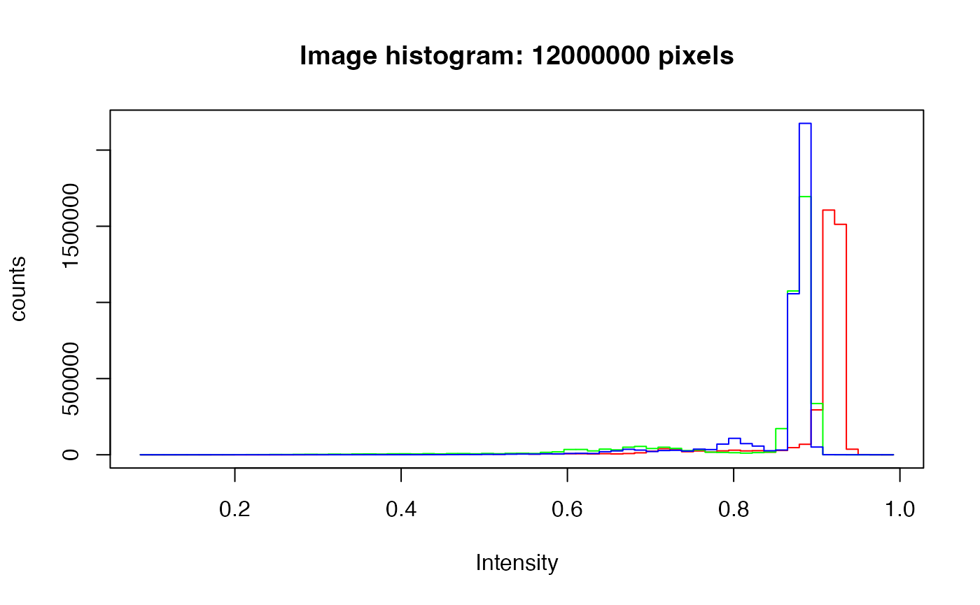
img2 <- img
colorMode(img2) <- Grayscale
display(img2, all = TRUE)

hist(img)

The tissue can be discerned with thresholding. The tall peak on the right is the background. The much lower peaks from around 0.6 to 0.85 must be the tissue. To capture the faint bluish region, the blue channel is used for thresholding. The threshold here is chosen based on the histogram and experimenting with nearby values.

mask <- img2[,,3] < 0.87
display(mask)

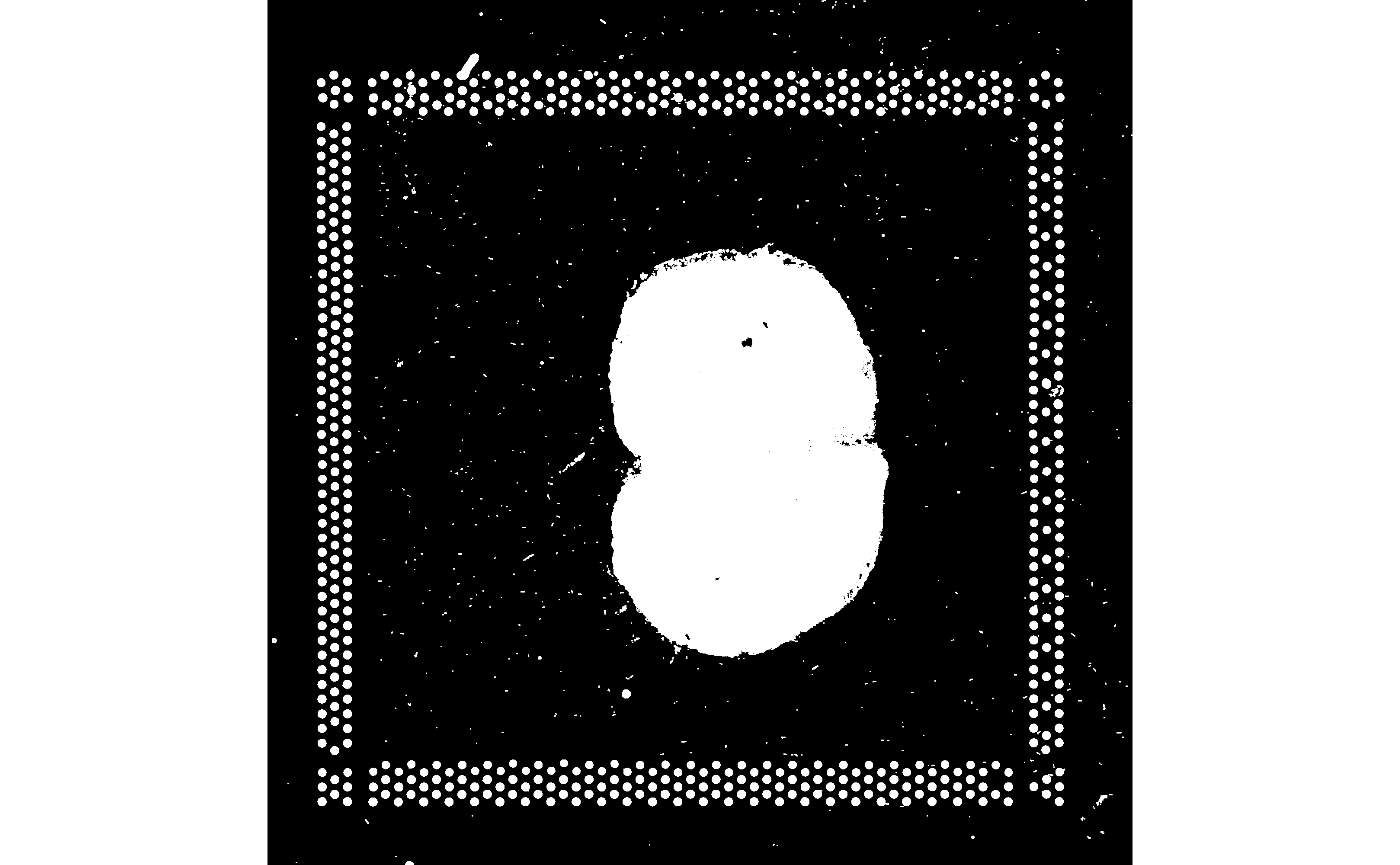
Then we use an opening operation (erosion followed by dilation) to denoise

kern <- makeBrush(3, shape='disc')
mask_open <- opening(mask, kern)
display(mask_open)

There are some small holes in the tissue, which can be removed by a closing operation (dilation followed by erosion):

mask_close <- closing(mask_open, kern)
display(mask_close)

There are some larger holes in the tissue mask, which may be real holes or faint regions with few nuclei missed by thresholding. They might not be large enough to affect which Visium spots intersect the tissue.

Now the main piece of tissue is clear. It must be the object with the largest area. However, there are two small pieces that should belong to the tissue at the top left. The debris and fiducials can be removed by setting all pixels in the mask outside the bounding box of the main piece to 0. Here we assign a different value to each contiguous object with bwlabel(), and use computeFeatures.shape() to find the area among other shape features (e.g. perimeter) of each object.

mask_label <- bwlabel(mask_close)
fts <- computeFeatures.shape(mask_label)
head(fts)
#>   s.area s.perimeter s.radius.mean s.radius.sd s.radius.min s.radius.max
#> 1     39          25      3.428773   1.3542219    1.4176036     5.762777
#> 2     20          14      2.032665   0.3439068    1.5000000     2.500000
#> 3      8           8      1.144123   0.4370160    0.7071068     1.581139
#> 4     14          10      1.689175   0.2160726    1.5811388     2.121320
#> 5     15          12      1.716761   0.4684015    1.0000000     2.236068
#> 6      9           8      1.207107   0.2071068    1.0000000     1.414214
summary(fts[,"s.area"])
#>     Min.  1st Qu.   Median     Mean  3rd Qu.     Max. 
#>      8.0     14.0     51.0    595.9    345.0 496326.0
max_ind <- which.max(fts[,"s.area"])
inds <- which(as.array(mask_label) == max_ind, arr.ind = TRUE)
head(inds)
#>       row col
#> [1,] 1168 562
#> [2,] 1169 562
#> [3,] 1170 562
#> [4,] 1158 563
#> [5,] 1159 563
#> [6,] 1160 563
row_inds <- c(seq_len(min(inds[,1])-1), seq(max(inds[,1])+1, nrow(mask_label), by = 1))
col_inds <- c(seq_len(min(inds[,2])-1), seq(max(inds[,2])+1, nrow(mask_label), by = 1))
mask_label[row_inds, ] <- 0
mask_label[,col_inds] <- 0
display(mask_label)

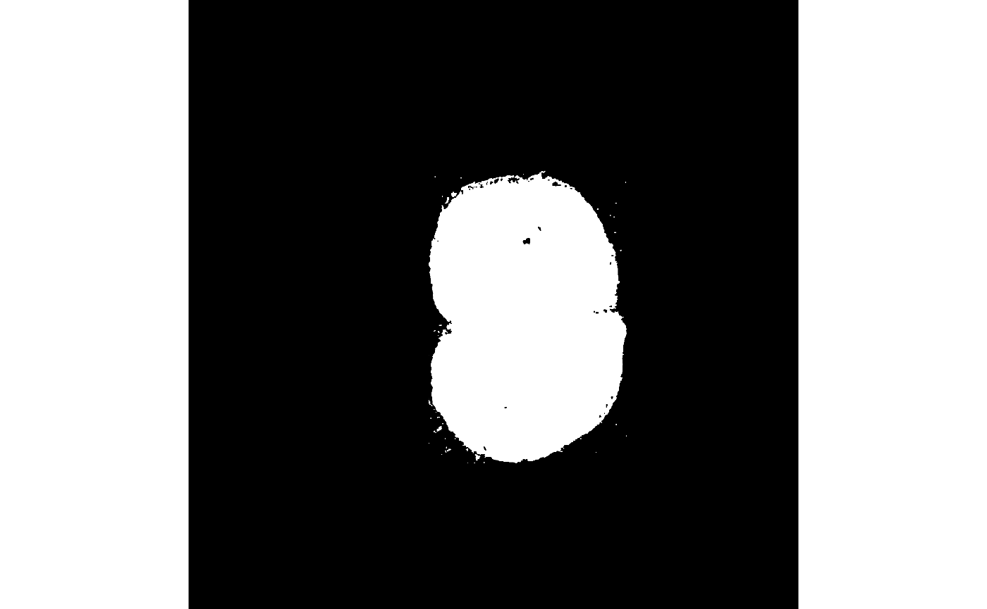
Then remove the small pieces that are debris.

unique(as.vector(mask_label))
#>  [1]   0 421 425 429 430 438 450 458 461 469 473 483 487 505 523 633 640 642 651
#> [20] 678 739 741 757 762 775 778 789 791 797 805 810 813 820 821 822 826 831 838
#> [39] 839 840 843 845 848 849 861 862 863
fts2 <- fts[unique(as.vector(mask_label))[-1],]
fts2 <- fts2[order(fts2[,"s.area"], decreasing = TRUE),]
plot(fts2[,1][-1], type = "l", ylab = "Area")

head(fts2, 10)
#>     s.area s.perimeter s.radius.mean s.radius.sd s.radius.min s.radius.max
#> 421 496326        3151    395.118732  68.6493949  234.1605637   485.715835
#> 450    217          55      7.840627   1.2883202    5.0010247    10.458197
#> 849    211          63      7.961248   2.0228566    3.8569142    12.189753
#> 797    182          56      7.547362   2.3368359    3.0772370    11.839919
#> 461    136          54      7.186020   3.2751628    0.9255555    12.479805
#> 741     92          56      6.365661   2.8382829    1.3273276    11.653219
#> 840     69          33      4.503526   1.6417370    1.6026264     7.076974
#> 862     63          37      4.854424   2.4445530    0.6361407     8.837838
#> 839     45          25      3.305562   0.7074306    1.9320455     4.526897
#> 775     32          22      2.887407   1.1755375    0.5300865     4.543636

Object number 797 is a piece of debris at the bottom left. The other pieces with area over 100 pixels are tissue. Since debris really is small bits of tissue, so the boundary between debris and tissue can be blurry. Here the two are distinguished by morphology on the H&E image and proximity to the main tissue.

#display(mask_label == 797)

Here we remove the debris from the mask

mask_label[mask_label %in% c(797, as.numeric(rownames(fts2)[fts2[,1] < 100]))] <- 0

Since most holes in the mask are faint regions of the tissue missed by thresholding, the holes will be filled

mask_label <- fillHull(mask_label)
display(paintObjects(mask_label, img, col=c("red", "yellow"), opac=c(1, 0.3)))

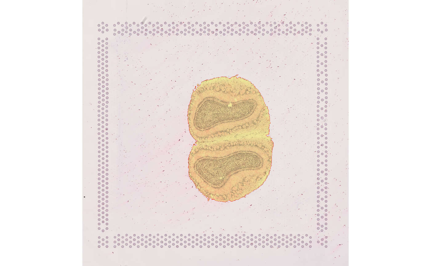
This segmentation process took a lot of manual oversight, in choosing the threshold, choosing kernel size and shape in the opening and closing operations, deciding whether to fill the holes, and deciding what is debris and what is tissue.

Convert tissue mask to polygon

Now we have the tissue mask, which we will convert to polygon. While OpenCV can directly perform the conversion, as there isn’t a comprehensive R wrapper of OpenCV, this conversion is more convoluted in R. We first convert the Image object to a raster as implemented in terra, the core R package for geospatial raster data. Then terra can convert the raster to polygon. As this image is downsized, the polygon will look quite pixelated. To mitigate this pixelation and save memory, the ms_simplify() function is used to simplify the polygon, only keeping a small proportion of all vertices. The st_simplify() function in sf can also simplify the polygons, but we can’t specify what proportion of vertices to keep.

raster2polygon <- function(seg, keep = 0.2) {
    r <- rast(as.array(seg), extent = ext(0, nrow(seg), 0, ncol(seg))) |> 
        trans() |> flip()
    r[r < 1] <- NA
    contours <- st_as_sf(as.polygons(r, dissolve = TRUE))
    simplified <- ms_simplify(contours, keep = keep)
    list(full = contours,
         simplified = simplified)
}
tb <- raster2polygon(mask_label)

Before adding the geometry to the SFE object, it needs to be scaled to match the coordinates of the spots

scale_factors <- fromJSON(file = "outs/spatial/scalefactors_json.json")
tb$simplified$geometry <- tb$simplified$geometry / scale_factors$tissue_hires_scalef
tissueBoundary(sfe) <- tb$simplified
plotSpatialFeature(sfe, "sum", annotGeometryName = "tissueBoundary", 
                   annot_fixed = list(fill = NA, color = "black"),
                   image_id = "lowres") +
    theme_void()

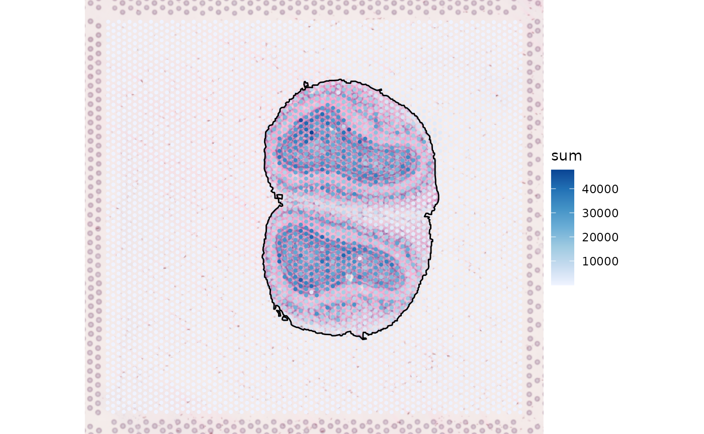
The mouse olfactory bulb is conventionally plotted horizontally. The entire SFE object can be transposed in histologial space to make the olfactory bulb horizontal.

sfe <- SpatialFeatureExperiment::transpose(sfe)
plotSpatialFeature(sfe, "sum", annotGeometryName = "tissueBoundary", 
                   annot_fixed = list(fill = NA, color = "black"),
                   image_id = "lowres")

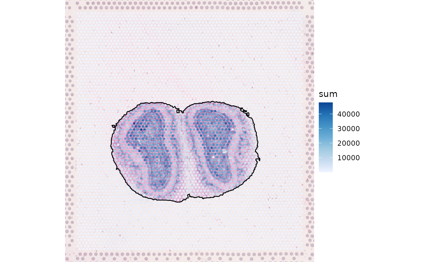
Then we can use geometric operations to find which spots intersect tissue, which spots are covered by tissue, and how much of each spot intersects tissue.

# Which spots intersect tissue
sfe$int_tissue <- annotPred(sfe, colGeometryName = "spotPoly", 
                            annotGeometryName = "tissueBoundary",
                            pred = st_intersects)
sfe$cov_tissue <- annotPred(sfe, colGeometryName = "spotPoly", 
                            annotGeometryName = "tissueBoundary",
                            pred = st_covered_by)

Discrepancies between Space Ranger’s annotation and the annotation based on tissue segmentation here:

sfe$diff_sr <- case_when(sfe$in_tissue == sfe$int_tissue ~ "same",
                         sfe$in_tissue & !sfe$int_tissue ~ "Space Ranger",
                         sfe$int_tissue & !sfe$in_tissue ~ "segmentation") |> 
    factor(levels = c("Space Ranger", "same", "segmentation"))
plotSpatialFeature(sfe, "diff_sr", 
                   annotGeometryName = "tissueBoundary", 
                   annot_fixed = list(fill = NA, size = 0.5, color = "black")) +
    scale_fill_brewer(type = "div", palette = 4)
#> Scale for fill is already present.
#> Adding another scale for fill, which will replace the existing scale.

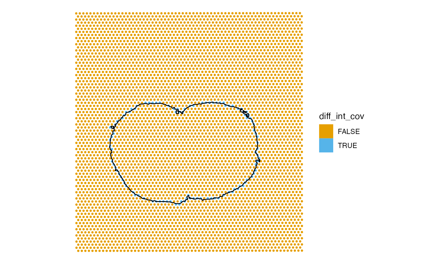
Spots at the margin can intersect the tissue without being covered by it.

sfe$diff_int_cov <- sfe$int_tissue != sfe$cov_tissue
plotSpatialFeature(sfe, "diff_int_cov", 
                   annotGeometryName = "tissueBoundary", 
                   annot_fixed = list(fill = NA, size = 0.5, color = "black"))

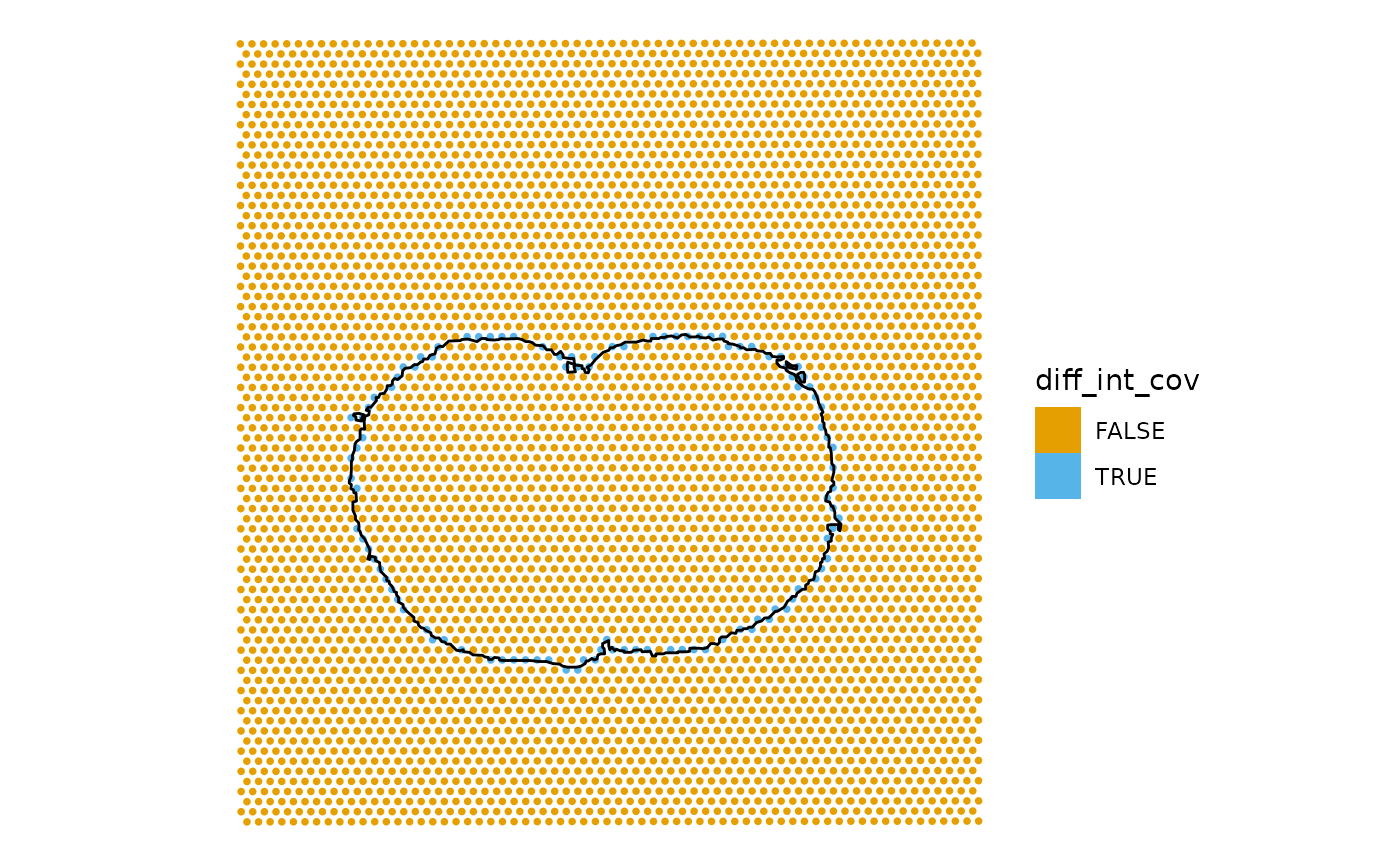
We can also get the geometries of the intersections between the tissue and the Visium spots, and then calculate what percentage of each spot is in tissue. However, this percentage may not be very useful if the tissue segmentation is subject to error. This percentage may be more useful for pathologist annotated histological regions or objects such as nuclei and myofibers.

spot_ints <- annotOp(sfe, colGeometryName = "spotPoly", 
                     annotGeometryName = "tissueBoundary", op = st_intersection)
sfe$pct_tissue <- st_area(spot_ints) / st_area(spotPoly(sfe)) * 100

For spots that intersect tissue, does total counts relate to percentage of the spot in tissue?

sfe_tissue <- sfe[,sfe$int_tissue]
plotColData(sfe_tissue, x = "pct_tissue", y = "sum", color_by = "diff_int_cov")

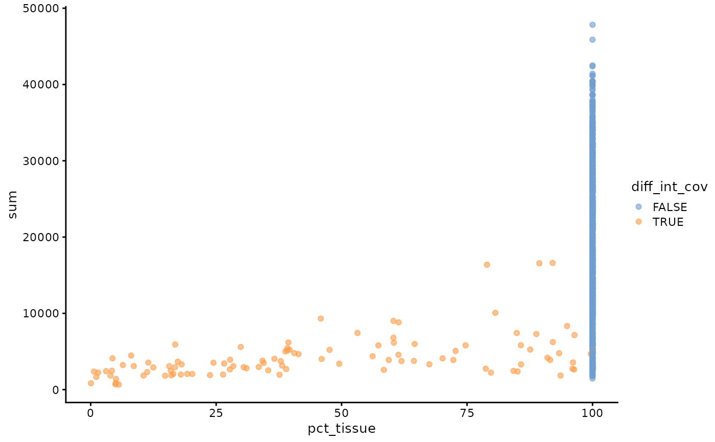
Spots that are not fully covered by tissue have lower total UMI counts, which can be due to both that they are not fully in tissue and the cell types with lower total counts in the histological region near the edge, as some spots fully covered by tissue also have low UMI counts.

Spatial autocorrelation of QC metrics

colGraph(sfe_tissue, "visium") <- findVisiumGraph(sfe_tissue)
qc_features <- c("sum", "detected", "subsets_mito_percent")
sfe_tissue <- colDataUnivariate(sfe_tissue, "moran.mc", qc_features, nsim = 200)
plotMoranMC(sfe_tissue, qc_features)

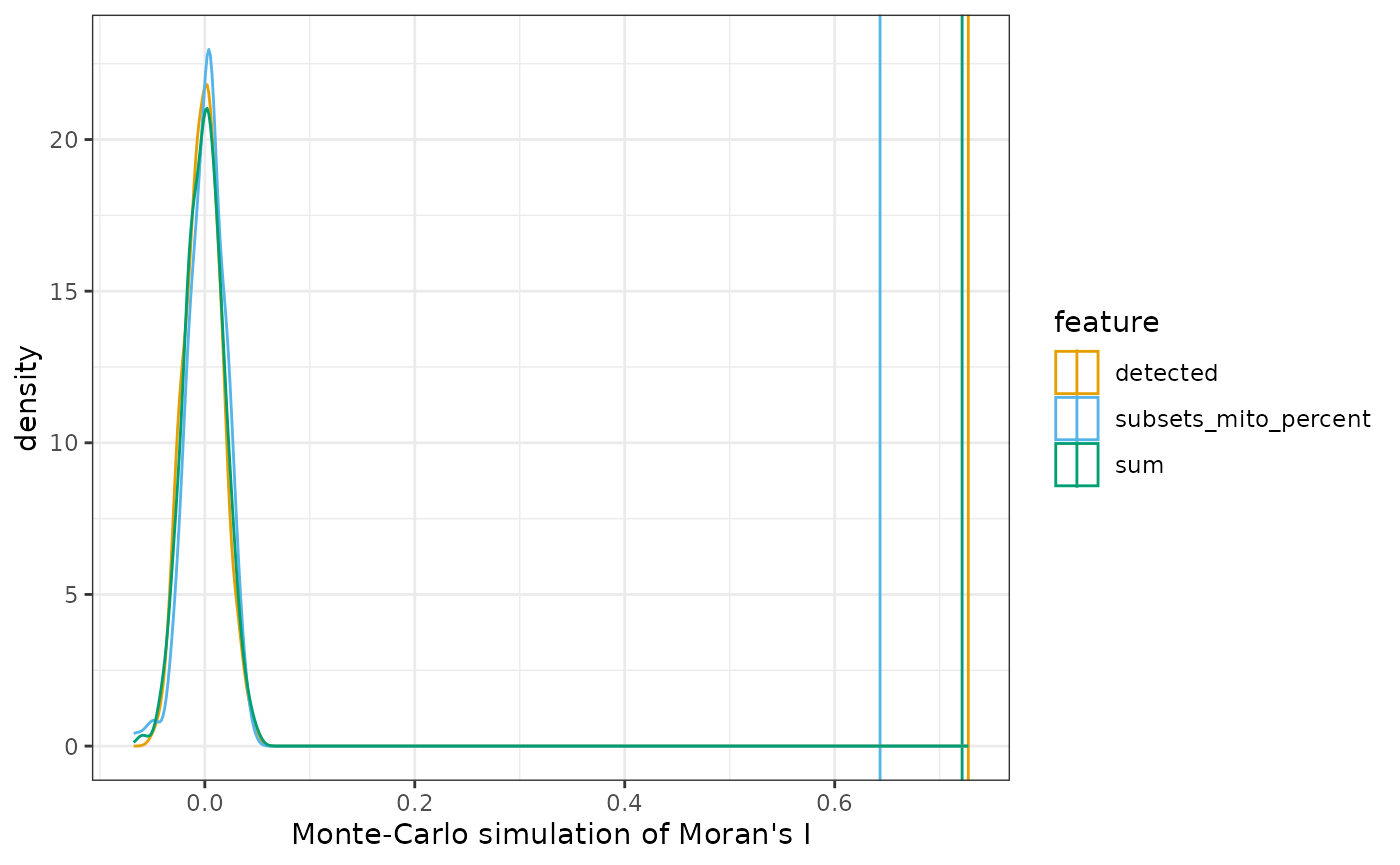
sfe_tissue <- colDataUnivariate(sfe_tissue, "sp.correlogram", qc_features,
                                order = 8)
plotCorrelogram(sfe_tissue, qc_features)

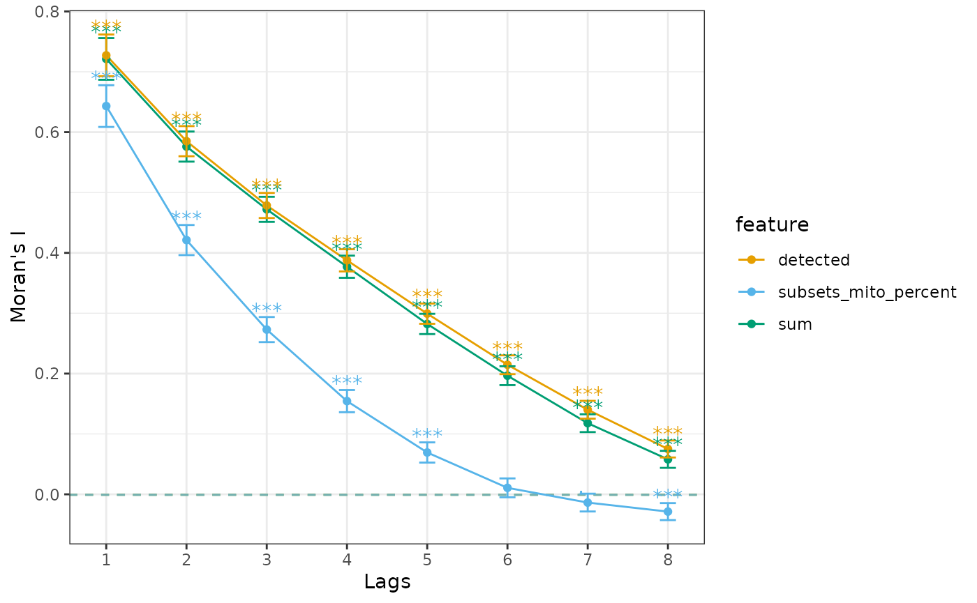
sfe_tissue <- colDataUnivariate(sfe_tissue, "localmoran", qc_features)
plotLocalResult(sfe_tissue, "localmoran", qc_features, ncol = 2,
                colGeometryName = "spotPoly", divergent = TRUE, 
                diverge_center = 0, image_id = "lowres", maxcell = 5e4)

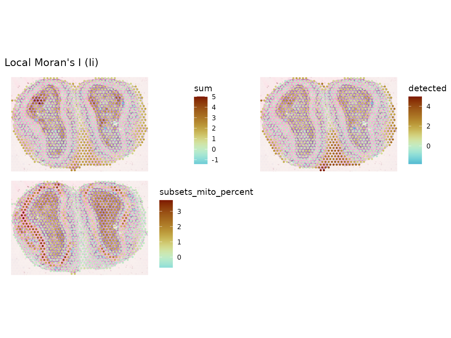
sfe_tissue <- colDataUnivariate(sfe_tissue, "LOSH", qc_features)
plotLocalResult(sfe_tissue, "LOSH", qc_features, ncol = 2,
                colGeometryName = "spotPoly", image_id = "lowres", maxcell = 5e4)

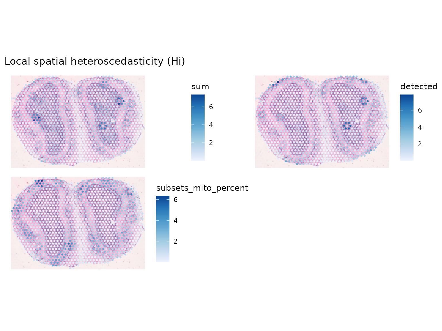
sfe_tissue <- colDataUnivariate(sfe_tissue, "moran.plot", qc_features)
moranPlot(sfe_tissue, "subsets_mito_percent")

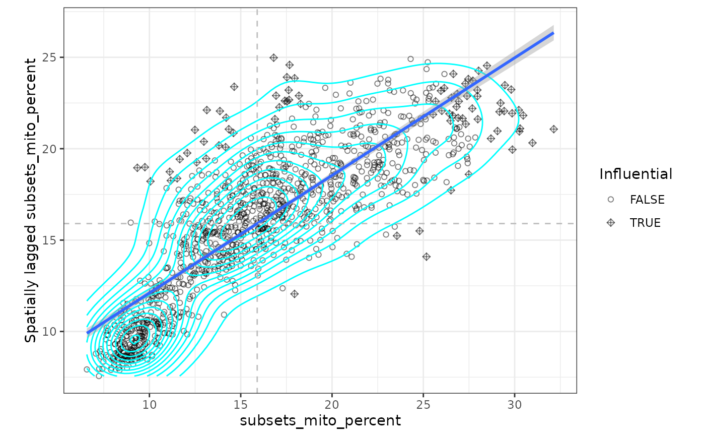
Spatial autocorrelation of gene expression

Normalize data with the scran method, and find highly variable genes

#clusters <- quickCluster(sfe_tissue)
#sfe_tissue <- computeSumFactors(sfe_tissue, clusters=clusters)
#sfe_tissue <- sfe_tissue[, sizeFactors(sfe_tissue) > 0]
sfe_tissue <- logNormCounts(sfe_tissue)
dec <- modelGeneVar(sfe_tissue)
hvgs <- getTopHVGs(dec, n = 2000)

Find Moran’s I for all highly variable genes:

sfe_tissue <- runMoransI(sfe_tissue, features = hvgs, BPPARAM = MulticoreParam(2))
plotRowDataHistogram(sfe_tissue, "moran_sample01")
#> Warning: Removed 30285 rows containing non-finite values (`stat_bin()`).

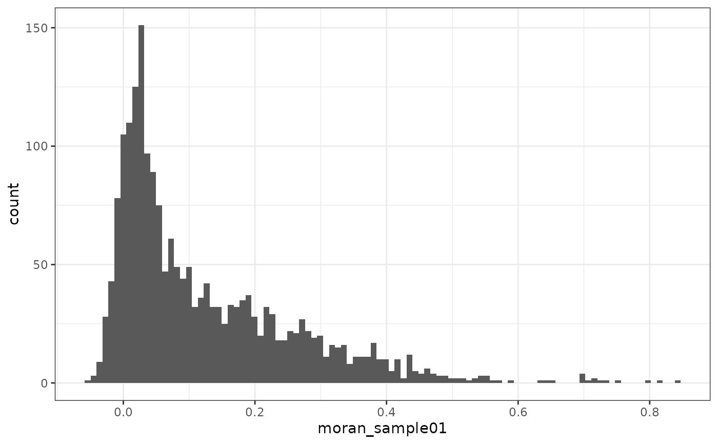
The vast majority of genes have positive Moran’s I. Here we’ll find the genes with the highest Moran’s I:

top_moran <- rownames(sfe_tissue)[order(rowData(sfe_tissue)$moran_sample01, 
                                        decreasing = TRUE)[1:9]]

We can use the gget info module from the gget package to get additional information on these genes, such as their descriptions, synonyms, transcripts and more from a collection of reference databases including Ensembl, UniProt and NCBI Here, we are showing their gene descriptions from NCBI:

gget_info <- gget$info(top_moran)

rownames(gget_info) <- gget_info$primary_gene_name
select(gget_info, ncbi_description)
#>                                                                                                                                                                                                                                                                                                                                                                                                                                                                                                                                                                                                                                                                                                         ncbi_description
#> S100a5                                                                                                                                                                                                                                                                                                                                                                                                                             Predicted to enable calcium-dependent protein binding activity; metal ion binding activity; and protein homodimerization activity. Located in neuronal cell body. Orthologous to human S100A5 (S100 calcium binding protein A5). [provided by Alliance of Genome Resources, Apr 2022]
#> Fabp7                                                                                                                                                                                                Predicted to enable fatty acid binding activity. Acts upstream of or within cell proliferation in forebrain; neurogenesis; and prepulse inhibition. Located in several cellular components, including cell projection; cell-cell junction; and neuronal cell body. Is expressed in several structures, including central nervous system; cranial nerve; gut; peripheral nervous system; and retina. Orthologous to human FABP7 (fatty acid binding protein 7). [provided by Alliance of Genome Resources, Apr 2022]
#> Apoe   This gene encodes a member of the apolipoprotein A1/A4/E family of proteins. This protein is involved in the transport of lipoproteins in the blood. It binds to a specific liver and peripheral cell receptor, and is essential for the normal catabolism of triglyceride-rich lipoprotein constituents. Homozygous knockout mice for this gene accumulate high levels of cholesterol in the blood and develop atherosclerosis. Different alleles of this gene have been associated with either increased risk or a protective effect for Alzheimer's disease in human patients. This gene maps to chromosome 7 in a cluster with the related apolipoprotein C1, C2 and C4 genes. [provided by RefSeq, Apr 2015]
#> Gng13                                                                                                                                                                                                                                                                                        Predicted to enable G-protein beta-subunit binding activity. Acts upstream of or within phospholipase C-activating G protein-coupled receptor signaling pathway and sensory perception of taste. Located in dendrite. Part of heterotrimeric G-protein complex. Is expressed in brain; gonad; gut; and liver. Orthologous to human GNG13 (G protein subunit gamma 13). [provided by Alliance of Genome Resources, Apr 2022]
#> Pcp4                                                      Enables calmodulin binding activity. Predicted to be involved in several processes, including calmodulin dependent kinase signaling pathway; negative regulation of protein kinase activity; and positive regulation of dopamine secretion. Predicted to be located in axon and neurofilament. Predicted to be part of protein-containing complex. Predicted to be active in cytoplasm. Is expressed in several structures, including alimentary system; central nervous system; genitourinary system; peripheral nervous system; and sensory organ. Orthologous to human PCP4 (Purkinje cell protein 4). [provided by Alliance of Genome Resources, Apr 2022]
#> Mtco2                                                                                                                                                                   Predicted to enable copper ion binding activity and oxidoreductase activity. Predicted to contribute to cytochrome-c oxidase activity. Predicted to be involved in ATP synthesis coupled electron transport; positive regulation of cellular biosynthetic process; and positive regulation of necrotic cell death. Located in mitochondrion. Is expressed in embryo; epiblast; heart; liver; and metanephros. Orthologous to several human genes including MTCO2P12 (MT-CO2 pseudogene 12). [provided by Alliance of Genome Resources, Apr 2022]
#> Ptgds                                                                                     Enables prostaglandin-D synthase activity and retinoid binding activity. Involved in prostaglandin biosynthetic process and regulation of circadian sleep/wake cycle, sleep. Acts upstream of or within negative regulation of male germ cell proliferation. Located in extracellular region. Is expressed in several structures, including alimentary system; genitourinary system; integumental system; nervous system; and sensory organ. Human ortholog(s) of this gene implicated in carotid artery disease. Orthologous to human PTGDS (prostaglandin D2 synthase). [provided by Alliance of Genome Resources, Apr 2022]
#> Mtnd4        Predicted to enable NADH dehydrogenase (ubiquinone) activity and ubiquinone binding activity. Predicted to contribute to NADH dehydrogenase activity. Predicted to be involved in several processes, including electron transport coupled proton transport; mitochondrial electron transport, NADH to ubiquinone; and mitochondrial respiratory chain complex I assembly. Located in mitochondrion. Human ortholog(s) of this gene implicated in Leber hereditary optic neuropathy; Parkinson's disease; macular degeneration; and schizophrenia. Orthologous to human MT-ND4 (mitochondrially encoded NADH:ubiquinone oxidoreductase core subunit 4). [provided by Alliance of Genome Resources, Apr 2022]

Plot the genes with the highest Moran’s I:

plotSpatialFeature(sfe_tissue, top_moran, ncol = 3, image_id = "lowres",
                   maxcell = 5e4, swap_rownames = "symbol")

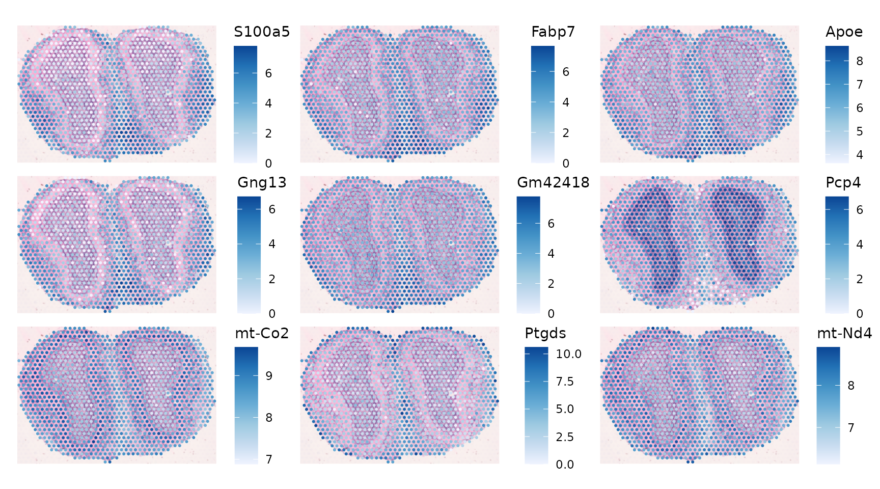
Here global Moran’s I seems to be more about tissue structure.

Some genes have negative Moran’s I that might not be statistically significant:

neg_moran <- rownames(sfe_tissue)[order(rowData(sfe_tissue)$moran_sample01, 
                                        decreasing = FALSE)[1:9]]
# Display NCBI descriptions for these genes
gget_info_neg <- gget$info(neg_moran)

rownames(gget_info_neg) <- gget_info_neg$primary_gene_name
select(gget_info_neg, ncbi_description)
#>                                                                                                                                                                                                                                                                                                                                                                                                                                                                                                                                                                                                                                                                                                                                                                                                                            ncbi_description
#> Hibch                                                                                                                                                                                                                                                                                                                                                                                                                                                                              Predicted to enable 3-hydroxyisobutyryl-CoA hydrolase activity. Predicted to be involved in valine catabolic process. Predicted to act upstream of or within branched-chain amino acid catabolic process. Located in mitochondrion. Orthologous to human HIBCH (3-hydroxyisobutyryl-CoA hydrolase). [provided by Alliance of Genome Resources, Apr 2022]
#> Syngr2                                                                                                                                                                                                                                                                                                                                                                                                                                           Predicted to be involved in regulated exocytosis and synaptic vesicle membrane organization. Predicted to act upstream of or within protein targeting. Located in synaptic vesicle. Is expressed in several structures, including genitourinary system; heart; liver; lung; and spleen. Orthologous to human SYNGR2 (synaptogyrin 2). [provided by Alliance of Genome Resources, Apr 2022]
#> Entpd5                                                                                                                                                                                                                                                                   Enables guanosine-diphosphatase activity and uridine-diphosphatase activity. Involved in several processes, including positive regulation of glycolytic process; protein N-linked glycosylation; and regulation of phosphatidylinositol 3-kinase signaling. Located in endoplasmic reticulum. Is expressed in several structures, including genitourinary system; gut; hemolymphoid system gland; liver; and nose. Orthologous to human ENTPD5 (ectonucleoside triphosphate diphosphohydrolase 5 (inactive)). [provided by Alliance of Genome Resources, Apr 2022]
#> Fyco1                                                                                                                                                                                                                                                            Predicted to enable metal ion binding activity. Predicted to be involved in plus-end-directed vesicle transport along microtubule and positive regulation of autophagosome maturation. Predicted to be located in Golgi apparatus. Predicted to be active in autophagosome; late endosome; and lysosome. Is expressed in central nervous system; early conceptus; and retina. Human ortholog(s) of this gene implicated in cataract 18. Orthologous to human FYCO1 (FYVE and coiled-coil domain autophagy adaptor 1). [provided by Alliance of Genome Resources, Apr 2022]
#> Ptpn18                                                                                                                                                                                                                                                                                                                                                                                             Enables non-membrane spanning protein tyrosine phosphatase activity. Acts upstream of or within blastocyst formation. Located in cytoplasm and nucleus. Is expressed in several structures, including alimentary system; brain; genitourinary system; immune system; and liver and biliary system. Orthologous to human PTPN18 (protein tyrosine phosphatase non-receptor type 18). [provided by Alliance of Genome Resources, Apr 2022]
#> Cbl                                                                                                                                                                                           Enables SH3 domain binding activity and ephrin receptor binding activity. Involved in regulation of platelet-derived growth factor receptor-alpha signaling pathway. Acts upstream of or within regulation of Rap protein signal transduction. Located in Golgi apparatus and cilium. Part of flotillin complex. Is expressed in male reproductive system and urinary system. Human ortholog(s) of this gene implicated in acute myeloid leukemia; juvenile myelomonocytic leukemia; lung non-small cell carcinoma; and myeloid neoplasm. Orthologous to human CBL (Cbl proto-oncogene). [provided by Alliance of Genome Resources, Apr 2022]
#> Dusp18  Predicted to enable protein tyrosine phosphatase activity and protein tyrosine/serine/threonine phosphatase activity. Predicted to be involved in peptidyl-threonine dephosphorylation and peptidyl-tyrosine dephosphorylation. Predicted to act upstream of or within protein targeting to membrane; protein targeting to mitochondrion; and response to antibiotic. Predicted to be located in mitochondrial inner membrane; mitochondrial intermembrane space; and nucleoplasm. Predicted to be extrinsic component of mitochondrial inner membrane and intrinsic component of mitochondrial inner membrane. Is expressed in central nervous system; dorsal root ganglion; olfactory epithelium; and retina. Orthologous to human DUSP18 (dual specificity phosphatase 18). [provided by Alliance of Genome Resources, Apr 2022]
#> Tsc22d3                                                                                                                                                                                                                                                        Enables MRF binding activity. Acts upstream of or within several processes, including negative regulation of activation-induced cell death of T cells; negative regulation of skeletal muscle tissue development; and negative regulation of transcription by RNA polymerase II. Located in cytoplasm and nucleus. Is expressed in several structures, including early conceptus; genitourinary system; nervous system; sensory organ; and viscerocranium. Orthologous to human TSC22D3 (TSC22 domain family member 3). [provided by Alliance of Genome Resources, Apr 2022]
#> Plekhg2                                                                                                                                                                                                                                                                                                                                                                                                                                                                                                                                                   Predicted to enable guanyl-nucleotide exchange factor activity. Predicted to be involved in regulation of actin filament polymerization. Orthologous to human PLEKHG2 (pleckstrin homology and RhoGEF domain containing G2). [provided by Alliance of Genome Resources, Apr 2022]
plotSpatialFeature(sfe_tissue, neg_moran, ncol = 3, swap_rownames = "symbol",
                   image_id = "lowres", maxcell = 5e4)

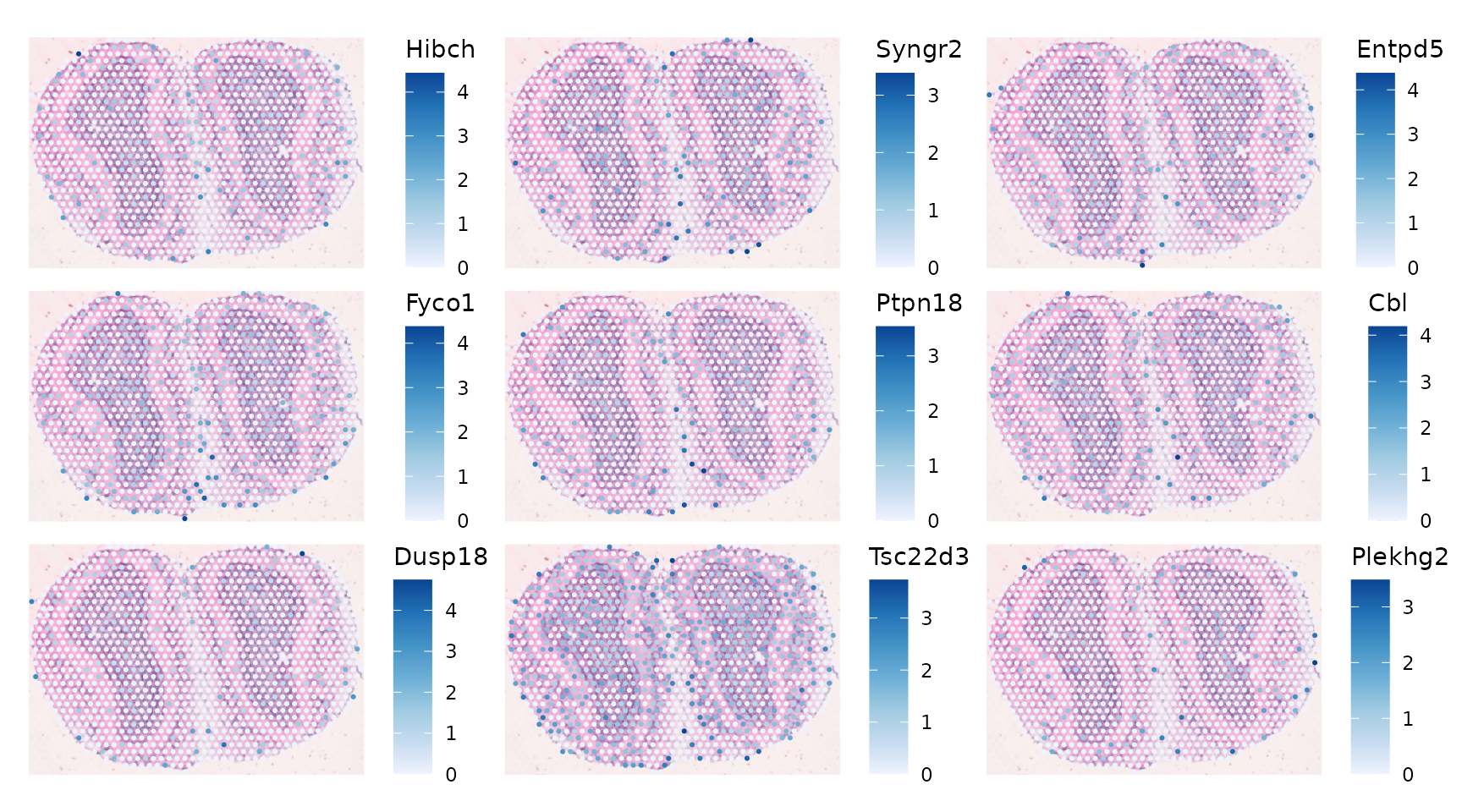
sfe_tissue <- runUnivariate(sfe_tissue, "moran.mc", neg_moran, 
                            colGraphName = "visium", nsim = 200, alternative = "less")
plotMoranMC(sfe_tissue, neg_moran, swap_rownames = "symbol")

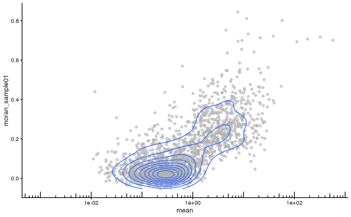
rowData(sfe_tissue)[neg_moran, c("moran_sample01", "moran.mc_p.value_sample01")]
#> DataFrame with 9 rows and 2 columns
#>                    moran_sample01 moran.mc_p.value_sample01
#>                         <numeric>                 <numeric>
#> ENSMUSG00000041426     -0.0531915                0.00497512
#> ENSMUSG00000048277     -0.0451179                0.00497512
#> ENSMUSG00000021236     -0.0445148                0.00497512
#> ENSMUSG00000025241     -0.0419121                0.00995025
#> ENSMUSG00000026126     -0.0399917                0.01990050
#> ENSMUSG00000034342     -0.0393964                0.00497512
#> ENSMUSG00000047205     -0.0381599                0.02487562
#> ENSMUSG00000031431     -0.0369456                0.02985075
#> ENSMUSG00000037552     -0.0368969                0.00995025

As there are 2000 highly variable genes and 2000 tests, these would no longer be significant after correcting for multiple testing.

Does global Moran’s I relate to gene expression level?

sfe_tissue <- addPerFeatureQCMetrics(sfe_tissue)
names(rowData(sfe_tissue))
#>  [1] "symbol"                                       
#>  [2] "Feature.Type"                                 
#>  [3] "I_sample01"                                   
#>  [4] "P.value_sample01"                             
#>  [5] "Adjusted.p.value_sample01"                    
#>  [6] "Feature.Counts.in.Spots.Under.Tissue_sample01"
#>  [7] "Median.Normalized.Average.Counts_sample01"    
#>  [8] "Barcodes.Detected.per.Feature_sample01"       
#>  [9] "moran_sample01"                               
#> [10] "K_sample01"                                   
#> [11] "moran.mc_statistic_sample01"                  
#> [12] "moran.mc_parameter_sample01"                  
#> [13] "moran.mc_p.value_sample01"                    
#> [14] "moran.mc_alternative_sample01"                
#> [15] "moran.mc_method_sample01"                     
#> [16] "moran.mc_res_sample01"                        
#> [17] "mean"                                         
#> [18] "detected"
plotRowData(sfe_tissue, x = "mean", y = "moran_sample01") +
    scale_x_log10() +
    annotation_logticks(sides = "b") +
    geom_density2d()
#> Warning: Transformation introduced infinite values in continuous x-axis
#> Transformation introduced infinite values in continuous x-axis
#> Warning: Removed 30285 rows containing non-finite values
#> (`stat_density2d()`).
#> Warning: Removed 30285 rows containing missing values (`geom_point()`).

Genes that are more highly expressed overall tend to have higher Moran’s I.

Apply spatial analysis methods to gene expression space

Spatial statistics that require a spatial neighborhood graph can also be applied to the k nearest neighbor graph not in histological space but in gene expression space. This is done in more depth in this vignette.

sfe_tissue <- runPCA(sfe_tissue, ncomponents = 30, subset_row = hvgs,
                     scale = TRUE) # scale as in Seurat
foo <- findKNN(reducedDim(sfe_tissue, "PCA")[,1:10], k=10, BNPARAM=AnnoyParam())
# Split by row
foo_nb <- asplit(foo$index, 1)
dmat <- 1/foo$distance
# Row normalize the weights
dmat <- sweep(dmat, 1, rowSums(dmat), FUN = "/")
glist <- asplit(dmat, 1)
# Sort based on index
ord <- lapply(foo_nb, order)
foo_nb <- lapply(seq_along(foo_nb), function(i) foo_nb[[i]][ord[[i]]])
class(foo_nb) <- "nb"
glist <- lapply(seq_along(glist), function(i) glist[[i]][ord[[i]]])

listw <- list(style = "W",
              neighbours = foo_nb,
              weights = glist)
class(listw) <- "listw"
attr(listw, "region.id") <- colnames(sfe_tissue)
colGraph(sfe_tissue, "knn10") <- listw
sfe_tissue <- runMoransI(sfe_tissue, features = hvgs, BPPARAM = MulticoreParam(2),
                         colGraphName = "knn10", name = "moran_ns")

Here we store the results in “moran_ns”, not to be confused with spatial Moran’s I results.

These are the genes that tend to be more similar to their neighbors in the 10 nearest neighbor graph in PCA space for gene expression rather than in histological space:

top_moran2 <- rownames(sfe_tissue)[order(rowData(sfe_tissue)$moran_ns_sample01, 
                                        decreasing = TRUE)[1:9]]
# Display NCBI descriptions for these genes
gget_info2 <- gget$info(top_moran2)

rownames(gget_info2) <- gget_info2$primary_gene_name
select(gget_info2, ncbi_description)
#>                                                                                                                                                                                                                                                                                                                                                                                                                                                                                                                                                                                                                                                                                                                                                                                                                                                                                                                                                                                                        ncbi_description
#> Mtco1                                                                                                                                                                                                                                                                                                                                                                                                                                                              Enables cytochrome-c oxidase activity. Predicted to be involved in electron transport coupled proton transport; mitochondrial electron transport, cytochrome c to oxygen; and response to oxidative stress. Located in mitochondrial inner membrane. Part of mitochondrial respiratory chain complex IV. Is expressed in several structures, including brown fat; heart; liver; metanephros; and skeletal muscle. Orthologous to human MT-CO1 (mitochondrially encoded cytochrome c oxidase I). [provided by Alliance of Genome Resources, Apr 2022]
#> Mtco2                                                                                                                                                                                                                                                                                                                                                                                                                                                                  Predicted to enable copper ion binding activity and oxidoreductase activity. Predicted to contribute to cytochrome-c oxidase activity. Predicted to be involved in ATP synthesis coupled electron transport; positive regulation of cellular biosynthetic process; and positive regulation of necrotic cell death. Located in mitochondrion. Is expressed in embryo; epiblast; heart; liver; and metanephros. Orthologous to several human genes including MTCO2P12 (MT-CO2 pseudogene 12). [provided by Alliance of Genome Resources, Apr 2022]
#> Apoe                                                                                                                                                                                                                                                                                                  This gene encodes a member of the apolipoprotein A1/A4/E family of proteins. This protein is involved in the transport of lipoproteins in the blood. It binds to a specific liver and peripheral cell receptor, and is essential for the normal catabolism of triglyceride-rich lipoprotein constituents. Homozygous knockout mice for this gene accumulate high levels of cholesterol in the blood and develop atherosclerosis. Different alleles of this gene have been associated with either increased risk or a protective effect for Alzheimer's disease in human patients. This gene maps to chromosome 7 in a cluster with the related apolipoprotein C1, C2 and C4 genes. [provided by RefSeq, Apr 2015]
#> Mtnd4                                                                                                                                                                                                                                                                                                       Predicted to enable NADH dehydrogenase (ubiquinone) activity and ubiquinone binding activity. Predicted to contribute to NADH dehydrogenase activity. Predicted to be involved in several processes, including electron transport coupled proton transport; mitochondrial electron transport, NADH to ubiquinone; and mitochondrial respiratory chain complex I assembly. Located in mitochondrion. Human ortholog(s) of this gene implicated in Leber hereditary optic neuropathy; Parkinson's disease; macular degeneration; and schizophrenia. Orthologous to human MT-ND4 (mitochondrially encoded NADH:ubiquinone oxidoreductase core subunit 4). [provided by Alliance of Genome Resources, Apr 2022]
#> Fabp7                                                                                                                                                                                                                                                                                                                                                                                                                                                                                               Predicted to enable fatty acid binding activity. Acts upstream of or within cell proliferation in forebrain; neurogenesis; and prepulse inhibition. Located in several cellular components, including cell projection; cell-cell junction; and neuronal cell body. Is expressed in several structures, including central nervous system; cranial nerve; gut; peripheral nervous system; and retina. Orthologous to human FABP7 (fatty acid binding protein 7). [provided by Alliance of Genome Resources, Apr 2022]
#> mt-Nd2                                                                                                                                                                                                                                                                                                                                                  Predicted to enable NADH dehydrogenase (ubiquinone) activity; ionotropic glutamate receptor binding activity; and protein kinase binding activity. Acts upstream of or within reactive oxygen species metabolic process. Located in mitochondrion. Is expressed in early conceptus and secondary oocyte. Human ortholog(s) of this gene implicated in Leber hereditary optic neuropathy; multiple sclerosis; myocardial infarction; neurodegenerative disease (multiple); and urinary bladder cancer. Orthologous to human MT-ND2 (mitochondrially encoded NADH:ubiquinone oxidoreductase core subunit 2). [provided by Alliance of Genome Resources, Apr 2022]
#> Ptn                                                                                                                                                                                                                                                                                                                                   Predicted to enable several functions, including glycosaminoglycan binding activity; signaling receptor binding activity; and syndecan binding activity. Involved in several processes, including decidualization; learning or memory; and regulation of nervous system development. Acts upstream of or within bone mineralization. Located in extracellular region. Is expressed in several structures, including alimentary system; genitourinary system; nervous system; respiratory system; and sensory organ. Human ortholog(s) of this gene implicated in adrenal carcinoma. Orthologous to human PTN (pleiotrophin). [provided by Alliance of Genome Resources, Apr 2022]
#> Apod                                                                                                                                                                                                                                                                                                                                                                               The protein encoded by this gene is a component of high-density lipoprotein (HDL), but is unique in that it shares greater structural similarity to lipocalin than to other members of the apolipoprotein family, and has a wider tissue expression pattern. The encoded protein is involved in lipid metabolism, and ablation of this gene results in defects in triglyceride metabolism. Elevated levels of this gene product have been observed in multiple tissues of Niemann-Pick disease mouse models, as well as in some tumors. Alternative splicing results in multiple transcript variants. [provided by RefSeq, Aug 2014]
#> Atp1a2 Predicted to enable several functions, including ATP binding activity; ATP hydrolysis activity; and alkali metal ion binding activity. Involved in several processes, including cellular response to steroid hormone stimulus; locomotory exploration behavior; and response to auditory stimulus. Acts upstream of or within several processes, including forebrain development; regulation of blood circulation; and regulation of muscle contraction. Located in T-tubule; cell projection; and neuronal cell body. Is expressed in several structures, including genitourinary system; heart; musculature; nervous system; and sensory organ. Used to study familial hemiplegic migraine 2. Human ortholog(s) of this gene implicated in alternating hemiplegia of childhood; benign neonatal seizures; familial hemiplegic migraine 2; hypertension; and migraine with aura. Orthologous to human ATP1A2 (ATPase Na+/K+ transporting subunit alpha 2). [provided by Alliance of Genome Resources, Apr 2022]
plotSpatialFeature(sfe_tissue, top_moran2, ncol = 3, swap_rownames = "symbol",
                   image_id = "lowres", maxcell = 5e4)

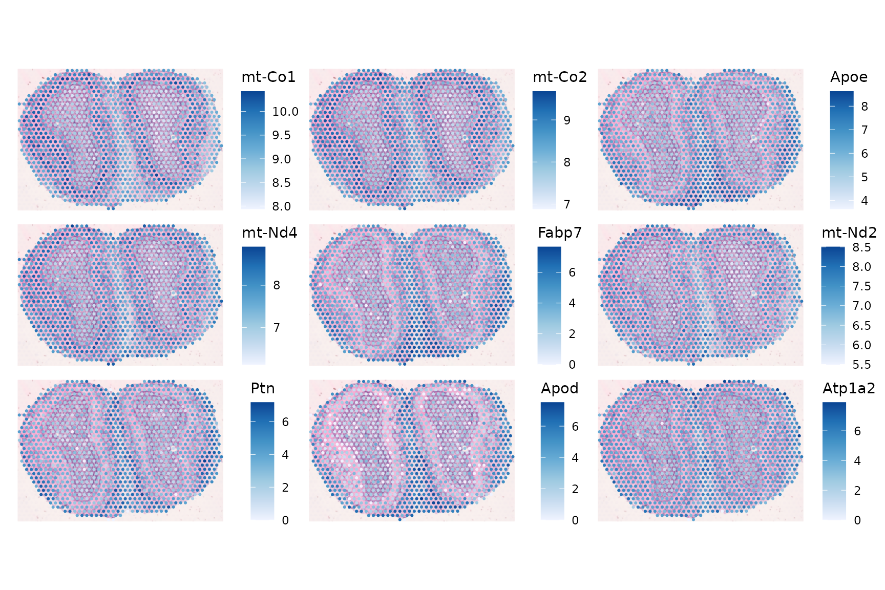
Although this Moran’s I was not computed in histological space, these genes with the highest Moran’s I in PCA space also show spatial structure, as different cell types reside in different spatial regions.

Session info

sessionInfo()
#> R version 4.3.2 (2023-10-31)
#> Platform: x86_64-apple-darwin20 (64-bit)
#> Running under: macOS Ventura 13.6
#> 
#> Matrix products: default
#> BLAS:   /Library/Frameworks/R.framework/Versions/4.3-x86_64/Resources/lib/libRblas.0.dylib 
#> LAPACK: /Library/Frameworks/R.framework/Versions/4.3-x86_64/Resources/lib/libRlapack.dylib;  LAPACK version 3.11.0
#> 
#> locale:
#> [1] en_US.UTF-8/en_US.UTF-8/en_US.UTF-8/C/en_US.UTF-8/en_US.UTF-8
#> 
#> time zone: UTC
#> tzcode source: internal
#> 
#> attached base packages:
#> [1] stats4    stats     graphics  grDevices utils     datasets  methods  
#> [8] base     
#> 
#> other attached packages:
#>  [1] reticulate_1.34.0              BiocNeighbors_1.20.0          
#>  [3] BiocParallel_1.36.0            dplyr_1.1.4                   
#>  [5] rmapshaper_0.5.0               sf_1.0-14                     
#>  [7] rlang_1.1.2                    terra_1.7-55                  
#>  [9] EBImage_4.44.0                 rjson_0.2.21                  
#> [11] bluster_1.12.0                 patchwork_1.1.3               
#> [13] stringr_1.5.1                  scran_1.30.0                  
#> [15] scater_1.30.0                  scuttle_1.12.0                
#> [17] ggplot2_3.4.4                  SingleCellExperiment_1.24.0   
#> [19] SummarizedExperiment_1.32.0    Biobase_2.62.0                
#> [21] GenomicRanges_1.54.1           GenomeInfoDb_1.38.1           
#> [23] IRanges_2.36.0                 S4Vectors_0.40.2              
#> [25] BiocGenerics_0.48.1            MatrixGenerics_1.14.0         
#> [27] matrixStats_1.1.0              SpatialFeatureExperiment_1.3.0
#> [29] Voyager_1.4.0                 
#> 
#> loaded via a namespace (and not attached):
#>   [1] RColorBrewer_1.1-3        jsonlite_1.8.7           
#>   [3] wk_0.9.0                  magrittr_2.0.3           
#>   [5] ggbeeswarm_0.7.2          magick_2.8.1             
#>   [7] farver_2.1.1              rmarkdown_2.25           
#>   [9] fs_1.6.3                  zlibbioc_1.48.0          
#>  [11] ragg_1.2.6                vctrs_0.6.4              
#>  [13] spdep_1.3-1               memoise_2.0.1            
#>  [15] DelayedMatrixStats_1.24.0 RCurl_1.98-1.13          
#>  [17] htmltools_0.5.7           S4Arrays_1.2.0           
#>  [19] curl_5.1.0                Rhdf5lib_1.24.0          
#>  [21] s2_1.1.4                  SparseArray_1.2.2        
#>  [23] rhdf5_2.46.0              sass_0.4.7               
#>  [25] spData_2.3.0              KernSmooth_2.23-22       
#>  [27] bslib_0.6.0               htmlwidgets_1.6.3        
#>  [29] desc_1.4.2                cachem_1.0.8             
#>  [31] igraph_1.5.1              lifecycle_1.0.4          
#>  [33] pkgconfig_2.0.3           rsvd_1.0.5               
#>  [35] Matrix_1.6-3              R6_2.5.1                 
#>  [37] fastmap_1.1.1             GenomeInfoDbData_1.2.11  
#>  [39] digest_0.6.33             colorspace_2.1-0         
#>  [41] ggnewscale_0.4.9          rprojroot_2.0.4          
#>  [43] dqrng_0.3.1               RSpectra_0.16-1          
#>  [45] irlba_2.3.5.1             textshaping_0.3.7        
#>  [47] beachmat_2.18.0           labeling_0.4.3           
#>  [49] fansi_1.0.5               mgcv_1.9-0               
#>  [51] abind_1.4-5               compiler_4.3.2           
#>  [53] proxy_0.4-27              withr_2.5.2              
#>  [55] tiff_0.1-11               viridis_0.6.4            
#>  [57] DBI_1.1.3                 highr_0.10               
#>  [59] R.utils_2.12.3            HDF5Array_1.30.0         
#>  [61] MASS_7.3-60               DelayedArray_0.28.0      
#>  [63] classInt_0.4-10           tools_4.3.2              
#>  [65] units_0.8-4               vipor_0.4.5              
#>  [67] beeswarm_0.4.0            R.oo_1.25.0              
#>  [69] glue_1.6.2                dbscan_1.1-11            
#>  [71] nlme_3.1-163              rhdf5filters_1.14.1      
#>  [73] grid_4.3.2                cluster_2.1.4            
#>  [75] generics_0.1.3            isoband_0.2.7            
#>  [77] gtable_0.3.4              R.methodsS3_1.8.2        
#>  [79] class_7.3-22              metapod_1.10.0           
#>  [81] BiocSingular_1.18.0       ScaledMatrix_1.10.0      
#>  [83] sp_2.1-2                  utf8_1.2.4               
#>  [85] XVector_0.42.0            ggrepel_0.9.4            
#>  [87] pillar_1.9.0              limma_3.58.1             
#>  [89] splines_4.3.2             lattice_0.22-5           
#>  [91] deldir_2.0-2              tidyselect_1.2.0         
#>  [93] locfit_1.5-9.8            knitr_1.45               
#>  [95] gridExtra_2.3             V8_4.4.0                 
#>  [97] edgeR_4.0.2               xfun_0.41                
#>  [99] statmod_1.5.0             DropletUtils_1.22.0      
#> [101] fftwtools_0.9-11          stringi_1.8.2            
#> [103] geojsonsf_2.0.3           yaml_2.3.7               
#> [105] boot_1.3-28.1             evaluate_0.23            
#> [107] codetools_0.2-19          tibble_3.2.1             
#> [109] cli_3.6.1                 systemfonts_1.0.5        
#> [111] munsell_0.5.0             jquerylib_0.1.4          
#> [113] Rcpp_1.0.11               png_0.1-8                
#> [115] parallel_4.3.2            pkgdown_2.0.7            
#> [117] jpeg_0.1-10               sparseMatrixStats_1.14.0 
#> [119] bitops_1.0-7              SpatialExperiment_1.12.0 
#> [121] viridisLite_0.4.2         scales_1.2.1             
#> [123] e1071_1.7-13              purrr_1.0.2              
#> [125] crayon_1.5.2              scico_1.5.0              
#> [127] cowplot_1.1.1