Python arguments are equivalent to long-option arguments (
--arg), unless otherwise specified. Flags are True/False arguments in Python. The manual for any gget tool can be called from the command-line using the-h--helpflag.
gget enrichr 💰
Perform an enrichment analysis on a list of genes using Enrichr or modEnrichr.
Return format: JSON (command-line) or data frame/CSV (Python).
Positional argument
genes
Short names (gene symbols) of genes to perform enrichment analysis on, e.g. PHF14 RBM3 MSL1 PHF21A.
Alternatively: use flag --ensembl to input a list of Ensembl gene IDs, e.g. ENSG00000106443 ENSG00000102317 ENSG00000188895.
Other required arguments
-db --database
Database database to use as reference for the enrichment analysis.
Supports any database listed here under 'Gene-set Library' or one of the following shortcuts:
'pathway' (KEGG_2021_Human)
'transcription' (ChEA_2016)
'ontology' (GO_Biological_Process_2021)
'diseases_drugs' (GWAS_Catalog_2019)
'celltypes' (PanglaoDB_Augmented_2021)
'kinase_interactions' (KEA_2015)
NOTE: database shortcuts are not supported for species other than 'human' or 'mouse'. Click on the species databases listed below under species to view a list of databases available for each species.
Optional arguments
-s --species
Species to use as reference for the enrichment analysis. (Default: human)
Options:
| Species | Database list |
|---|---|
human | Enrichr |
mouse | Equivalent to human |
fly | FlyEnrichr |
yeast | YeastEnrichr |
worm | WormEnrichr |
fish | FishEnrichr |
-bkg_l --background_list
Short names (gene symbols) of background genes to perform enrichment analysis on, e.g. NSUN3 POLRMT NLRX1.
Alternatively: use flag --ensembl_background to input a list of Ensembl gene IDs.
See this Tweetorial to learn why you should use a background gene list when performing an enrichment analysis.
-o --out
Path to the file the results will be saved in, e.g. path/to/directory/results.csv (or .json). (Default: Standard out.)
Python: save=True will save the output in the current working directory.
-ko --kegg_out
Path to the png file the marked KEGG pathway images will be saved in, e.g. path/to/directory/pathway.png. (Default: None)
-kr --kegg_rank
Rank of the KEGG pathway to be plotted. (Default: 1)
figsize
Python only. (width, height) of plot in inches. (Default: (10,10))
ax
Python only. Pass a matplotlib axes object for plot customization. (Default: None)
Flags
-e --ensembl
Add this flag if genes are given as Ensembl gene IDs.
-e_b --ensembl_bkg
Add this flag if background_list are given as Ensembl gene IDs.
-bkg --background
If True, use set of > 20,000 default background genes listed here.
-csv --csv
Command-line only. Returns results in CSV format.
Python: Use json=True to return output in JSON format.
-q --quiet
Command-line only. Prevents progress information from being displayed.
Python: Use verbose=False to prevent progress information from being displayed.
plot
Python only. plot=True provides a graphical overview of the first 15 results (default: False).
Examples
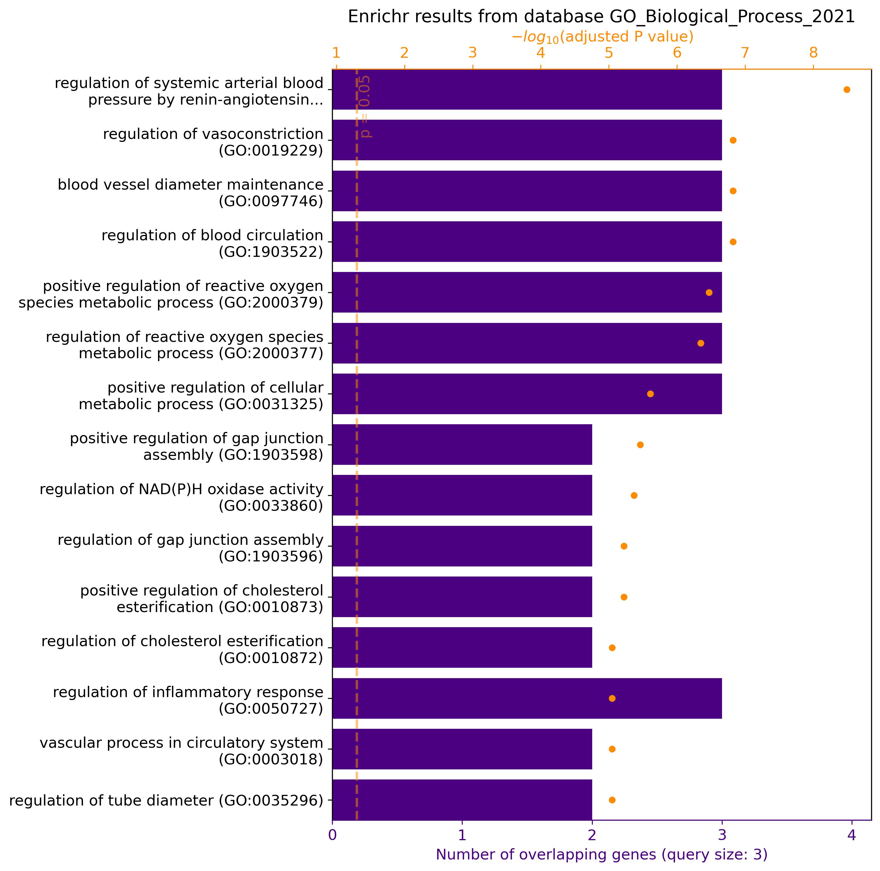
gget enrichr -db ontology ACE2 AGT AGTR1
# Python
gget.enrichr(["ACE2", "AGT", "AGTR1"], database="ontology", plot=True)
→ Returns pathways/functions involving genes ACE2, AGT, and AGTR1 from the GO Biological Process 2021 database. In Python, plot=True returns a graphical overview of the results:
Use gget enrichr with a background gene list:
See this Tweetorial to learn why you should use a background gene list when performing an enrichment analysis.
# Here, we are passing the input genes first (positional argument 'genes'), so they are not added to the background gene list behind the '-bkgr_l' argument
gget enrichr \
PHF14 RBM3 MSL1 PHF21A ARL10 INSR JADE2 P2RX7 LINC00662 CCDC101 PPM1B KANSL1L CRYZL1 ANAPC16 TMCC1 CDH8 RBM11 CNPY2 HSPA1L CUL2 PLBD2 LARP7 TECPR2 ZNF302 CUX1 MOB2 CYTH2 SEC22C EIF4E3 ROBO2 ADAMTS9-AS2 CXXC1 LINC01314 ATF7 ATP5F1 \
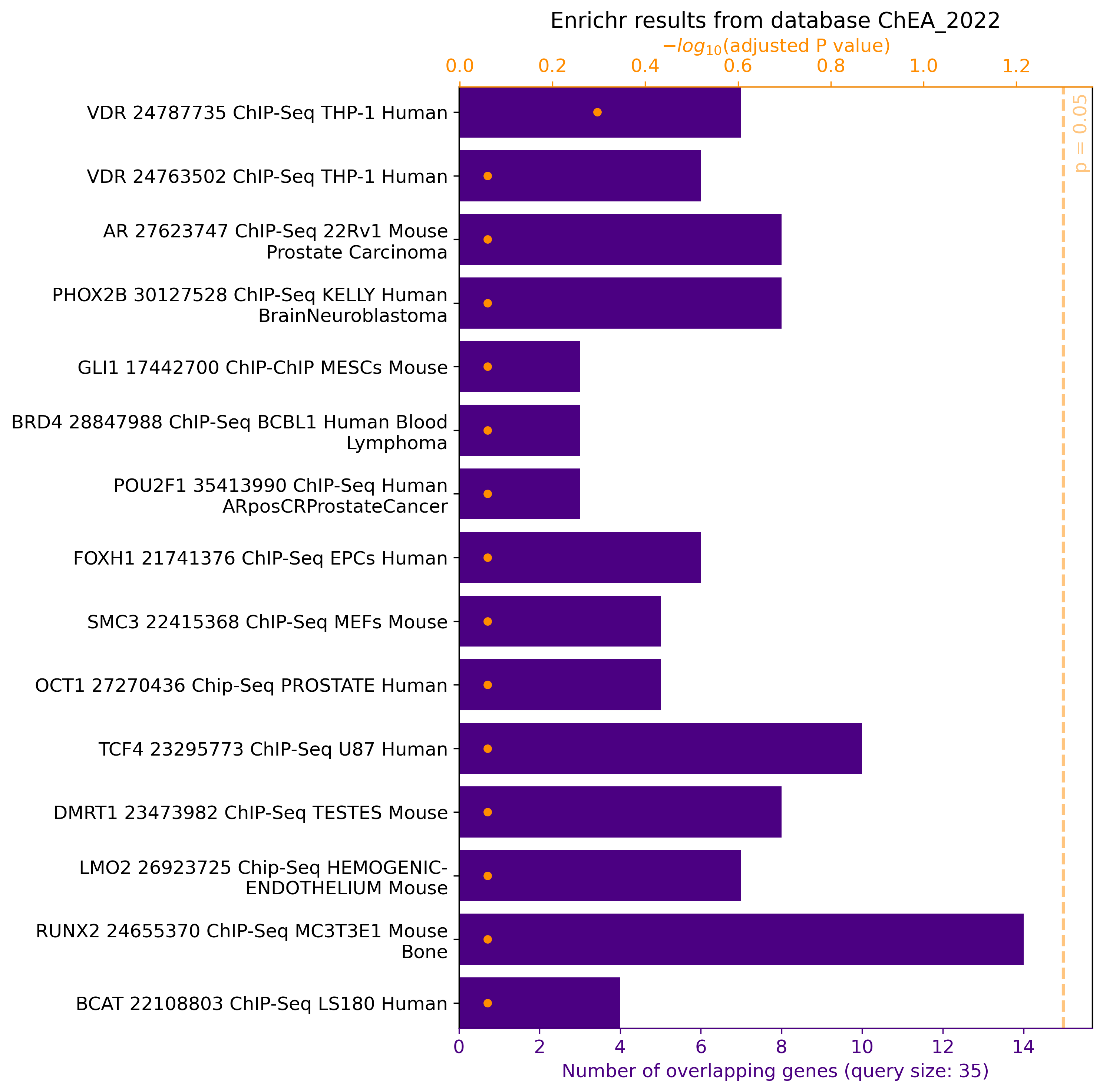
-db ChEA_2022 \
-bkg_l NSUN3 POLRMT NLRX1 SFXN5 ZC3H12C SLC25A39 ARSG DEFB29 PCMTD2 ACAA1A LRRC1 2810432D09RIK SEPHS2 SAC3D1 TMLHE LOC623451 TSR2 PLEKHA7 GYS2 ARHGEF12 HIBCH LYRM2 ZBTB44 ENTPD5 RAB11FIP2 LIPT1 INTU ANXA13 KLF12 SAT2 GAL3ST2 VAMP8 FKBPL AQP11 TRAP1 PMPCB TM7SF3 RBM39 BRI3 KDR ZFP748 NAP1L1 DHRS1 LRRC56 WDR20A STXBP2 KLF1 UFC1 CCDC16 9230114K14RIK RWDD3 2610528K11RIK ACO1 CABLES1 LOC100047214 YARS2 LYPLA1 KALRN GYK ZFP787 ZFP655 RABEPK ZFP650 4732466D17RIK EXOSC4 WDR42A GPHN 2610528J11RIK 1110003E01RIK MDH1 1200014M14RIK AW209491 MUT 1700123L14RIK 2610036D13RIK PHF14 RBM3 MSL1 PHF21A ARL10 INSR JADE2 P2RX7 LINC00662 CCDC101 PPM1B KANSL1L CRYZL1 ANAPC16 TMCC1 CDH8 RBM11 CNPY2 HSPA1L CUL2 PLBD2 LARP7 TECPR2 ZNF302 CUX1 MOB2 CYTH2 SEC22C EIF4E3 ROBO2 ADAMTS9-AS2 CXXC1 LINC01314 ATF7 ATP5F1COX15 TMEM30A NSMCE4A TM2D2 RHBDD3 ATXN2 NFS1 3110001I20RIK BC038156 C330002I19RIK ZFYVE20 POLI TOMM70A LOC100047782 2410012H22RIK RILP A230062G08RIK PTTG1IP RAB1 AFAP1L1 LYRM5 2310026E23RIK SLC7A6OS MAT2B 4932438A13RIK LRRC8A SMO NUPL2
# Python
gget.enrichr(
	genes = [
		"PHF14", "RBM3", "MSL1", "PHF21A", "ARL10", "INSR", "JADE2", "P2RX7",
		"LINC00662", "CCDC101", "PPM1B", "KANSL1L", "CRYZL1", "ANAPC16", "TMCC1",
		"CDH8", "RBM11", "CNPY2", "HSPA1L", "CUL2", "PLBD2", "LARP7", "TECPR2",
		"ZNF302", "CUX1", "MOB2", "CYTH2", "SEC22C", "EIF4E3", "ROBO2",
		"ADAMTS9-AS2", "CXXC1", "LINC01314", "ATF7", "ATP5F1"
	],
	database = "ChEA_2022",
	background_list = [
		"NSUN3","POLRMT","NLRX1","SFXN5","ZC3H12C","SLC25A39","ARSG",
		"DEFB29","PCMTD2","ACAA1A","LRRC1","2810432D09RIK","SEPHS2",
		"SAC3D1","TMLHE","LOC623451","TSR2","PLEKHA7","GYS2","ARHGEF12",
		"HIBCH","LYRM2","ZBTB44","ENTPD5","RAB11FIP2","LIPT1",
		"INTU","ANXA13","KLF12","SAT2","GAL3ST2","VAMP8","FKBPL",
		"AQP11","TRAP1","PMPCB","TM7SF3","RBM39","BRI3","KDR","ZFP748",
		"NAP1L1","DHRS1","LRRC56","WDR20A","STXBP2","KLF1","UFC1",
		"CCDC16","9230114K14RIK","RWDD3","2610528K11RIK","ACO1",
		"CABLES1", "LOC100047214","YARS2","LYPLA1","KALRN","GYK",
		"ZFP787","ZFP655","RABEPK","ZFP650","4732466D17RIK","EXOSC4",
		"WDR42A","GPHN","2610528J11RIK","1110003E01RIK","MDH1","1200014M14RIK",
		"AW209491","MUT","1700123L14RIK","2610036D13RIK",
		"PHF14", "RBM3", "MSL1", "PHF21A", "ARL10", "INSR", "JADE2",
		"P2RX7", "LINC00662", "CCDC101", "PPM1B", "KANSL1L", "CRYZL1",
		"ANAPC16", "TMCC1","CDH8", "RBM11", "CNPY2", "HSPA1L", "CUL2",
		"PLBD2", "LARP7", "TECPR2", "ZNF302", "CUX1", "MOB2", "CYTH2",
		"SEC22C", "EIF4E3", "ROBO2", "ADAMTS9-AS2", "CXXC1", "LINC01314", "ATF7",
		"ATP5F1""COX15","TMEM30A","NSMCE4A","TM2D2","RHBDD3","ATXN2","NFS1",
		"3110001I20RIK","BC038156","C330002I19RIK","ZFYVE20","POLI","TOMM70A",
		"LOC100047782","2410012H22RIK","RILP","A230062G08RIK",
		"PTTG1IP","RAB1","AFAP1L1", "LYRM5","2310026E23RIK",
		"SLC7A6OS","MAT2B","4932438A13RIK","LRRC8A","SMO","NUPL2"
	],
	plot=True
)
→ Returns hits of the input gene list given the background gene list from the transcription factor/target library ChEA 2022. In Python, plot=True returns a graphical overview of the results:
Generate a KEGG pathway image with the genes from the enrichment analysis highlighted:
This feature is available thanks to a PR by Noriaki Sato.
gget enrichr -db pathway --kegg_out kegg.png --kegg_rank 1 ZBP1 IRF3 RIPK1
# Python
gget.enrichr(["ZBP1", "IRF3", "RIPK1"], database="pathway", kegg_out="kegg.png", kegg_rank=1)
→ In addition to the standard gget enrichr output, the kegg_out argument saves an image with the genes from the enrichment analysis highlighted in the KEGG pathway:
The following example was submitted by Dylan Lawless via PR:
Use gget enrichr in R and create a similar plot using ggplot.
NOTE the switch of axes compared to the Python plot.
system("pip install gget")
install.packages("reticulate")
library(reticulate)
gget <- import("gget")

# Perform enrichment analysis on a list of genes
df <- gget$enrichr(list("ACE2", "AGT", "AGTR1"), database = "ontology")

# Count number of overlapping genes
df$overlapping_genes_count <- lapply(df$overlapping_genes, length) |> as.numeric()

# Only keep the top 15 results
df <- df[1:15, ]

# Plot
library(ggplot2)

df |>
	ggplot() +
	geom_bar(aes(
		x = -log10(adj_p_val),
		y = reorder(path_name, -adj_p_val)
	),
	stat = "identity",
  	fill = "lightgrey",
  	width = 0.5,
	color = "black") +
	geom_text(
		aes(
			y = path_name,
			x = (-log10(adj_p_val)),
			label = overlapping_genes_count
		),
		nudge_x = 0.75,
		show.legend = NA,
		color = "red"
	) +
  	geom_text(
		aes(
			y = Inf,
			x = Inf,
      			hjust = 1,
      			vjust = 1,
			label = "# of overlapping genes"
		),
		show.legend = NA,
		color = "red"
	) +
	geom_vline(linetype = "dotted", linewidth = 1, xintercept = -log10(0.05)) +
	ylab("Pathway name") +
	xlab("-log10(adjusted P value)")
Tutorials
Using gget enrichr with background genes
References
If you use gget enrichr in a publication, please cite the following articles:
-
Luebbert, L., & Pachter, L. (2023). Efficient querying of genomic reference databases with gget. Bioinformatics. https://doi.org/10.1093/bioinformatics/btac836
-
Chen EY, Tan CM, Kou Y, Duan Q, Wang Z, Meirelles GV, Clark NR, Ma'ayan A. Enrichr: interactive and collaborative HTML5 gene list enrichment analysis tool. BMC Bioinformatics. 2013; 128(14). https://doi.org/10.1186/1471-2105-14-128
-
Kuleshov MV, Jones MR, Rouillard AD, Fernandez NF, Duan Q, Wang Z, Koplev S, Jenkins SL, Jagodnik KM, Lachmann A, McDermott MG, Monteiro CD, Gundersen GW, Ma'ayan A. Enrichr: a comprehensive gene set enrichment analysis web server 2016 update. Nucleic Acids Research. 2016; gkw377. doi: 10.1093/nar/gkw377
-
Xie Z, Bailey A, Kuleshov MV, Clarke DJB., Evangelista JE, Jenkins SL, Lachmann A, Wojciechowicz ML, Kropiwnicki E, Jagodnik KM, Jeon M, & Ma’ayan A. Gene set knowledge discovery with Enrichr. Current Protocols, 1, e90. 2021. doi: 10.1002/cpz1.90.
If working with non-human/mouse datasets, please also cite:
- Kuleshov MV, Diaz JEL, Flamholz ZN, Keenan AB, Lachmann A, Wojciechowicz ML, Cagan RL, Ma'ayan A. modEnrichr: a suite of gene set enrichment analysis tools for model organisms. Nucleic Acids Res. 2019 Jul 2;47(W1):W183-W190. doi: 10.1093/nar/gkz347. PMID: 31069376; PMCID: PMC6602483.